Brief discussions on uncertainty contributors of GNSS-based positioning (Part 2)
In this post, we will start from the highest view of how we can estimate a position from at least four GNSS satellite ranging signals.
In this post, we will start from the highest view of how we can estimate a position from at least four GNSS satellite ranging signals.
This highest view is represented in the final navigation equations where the main variables are presented.
These main variables are pseudorange, satellite locations $X,Y,Z$ coordinates and systematic receiver clock error. The previous two variables need to be estimated from GNSS signals and the later one is the byproduct of solving the navigation equation.
From this view, we can derive the main uncertainty contributors of GNSS position measurements at the highest-level variables.
Later, we will breakdown these main contributors into smaller contributors that constitute the calculation of the main variables in the navigation equations.
READ MORE: Brief discussions on uncertainty contributors of GNSS-based positioning (Part 1)
Navigation equation formation
To have a position, we need to have at least four GNSS satellites in view. The reason is that, there are four variables to solve, the three coordinate location ($X,Y,Z $)-coordinate of a receiver and the receiver clock offset (with respect to the GNSS system time) [1,2,3,4].
However, to have an averaging effect to reduce errors from many sources, we will require five or more GNSS satellites in view to calculate the receiver position. That is to make the system of equations to be over-determined.
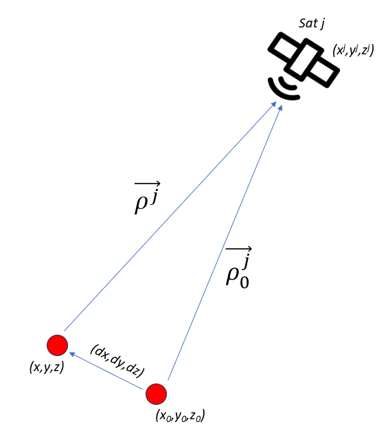
Figure 1 shows the illustration of the requirement of at least four GNSS satellites in-view to estimate the location of a receiver. In figure 1, the two main variables constituting a navigation equations are shown: pseudorange $\rho$ and satellite $X,Y,Z$-locations.
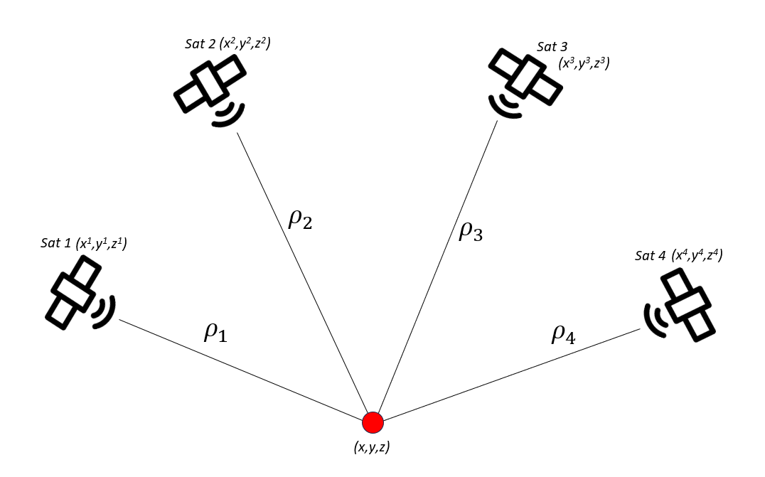
The navigation equation is a set of pseudorange calculations between a receiver and GNSS satellites. It is called pseudorange since there is a systematic receiver clock error that causes the calculated distance between a satellite to the receiver is not the real range yet [1,2].
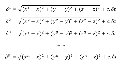
An estimated pseudorange $\hat{\rho} ^{i}$ is calculated as follows:
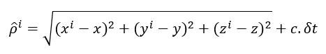
Where $\hat{\rho} ^{i}$ is the pseudorange between a receiver and satellite $i$, $x^{i}, y^{i}, z^{i}$ are the coordinate of the satellite $i$ and $x,y,z$ are the coordinate of the receiver. The receiver clock-bias $\delta t$ is constant and systematic for all the set of pseudorange equations.
Pseudorange is calculated from the time of flight multiplied with the speed of light. Time of flight is the travel time required for the ranging signal from being transmitted from a GNSS satellite to the receiver.
From the pseudorange calculation, we can identify that this time of flight is affected by many variables (phenomenon), that are delay in the ionospheric layer, delay in the tropospheric layer, multipath from environment, satellite clock-bias, signal processing to locate the first sample of the ranging signal (GNSS signal) that arrives at the receiver, satellite locations and other factors.
Satellite $x,y,z$-coordinate or orbit is computed from the broadcasted ephemeris messages in GNSS signals. The broadcasted ephemeris requires GNSS signal demodulation process. The satellite orbit will be affected by dynamic disturbances from external factors, such as solar pressure, space debris and gravitational forces from the Moon and the Sun.
Those variables or factors affecting both pseudorange and satellite coordinate or orbit are considered as relevant uncertainty contributors on GNSS position measurements.
The set of navigation equations can be written as:
From the above navigation equations, we can see that the equation is non-linear. There are options to solve this set of equations, such as:
- Finding a closed-form solution. This solution is complicated to solve in closed-form solutions. Also, in the closed-form solution we cannot get deep meaningful insight about the geometrical relations between a receiver and satellite in view.
- Using an iterative non-linear optimisation. This non-linear optimisation/iterative solution may not always give optimal solutions (depending on some factors such as good initial solution estimate, iterative steps, number of iterative steps and others)
Both of these solutions are still complex. To get a practical solution, a linearisation process based on Taylor-expansion is applied to the set of navigation equations.
Linearisation of navigation equation
The linearisation process is performed by applying Taylor-series approximation on the pseudorange $\rho$ calculation at around the neighbour of a point $(x_{0}, y_{0},z_{0})$, as the approximate position of a receiver, and is expected to be “close” to the real position of the receiver [3].
Figure 2 shows the illustration of the linearisation process of the pseudorange $\rho$ geometric equation. To get the linear equation, the Taylor series approximation applied to the pseudorange equation is truncated up to order one.
As a refresher, one-variable Taylor-series expansion can be written as follows:
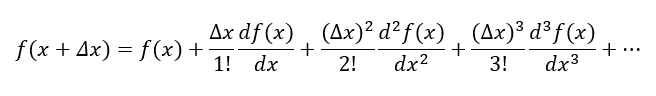
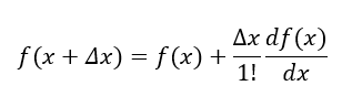
The above Taylor-series can be used to linearise the function $f(x)$ at around $x=a$ by neglecting the higher order of the series (> order 2), such that the series becomes:
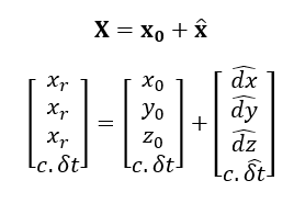
From figure 2 above, we can write the receiver true location, in a matrix form, as:
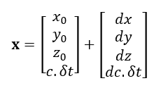
Hence, we can re-write the function of a receiver locations as:

The Taylor-series expansion up to order one of the equation above is written as follows:
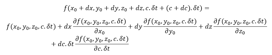
Hence,
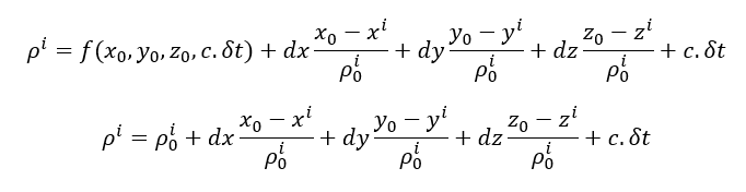
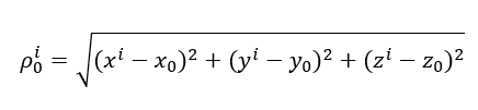
Where:
READ MORE: Measurement uncertainty estimation: Spreadsheets method
Solving navigation equation
To calculate GNSS positioning, we need construct a set of navigation equations as a set of pseudorange equations as follows:
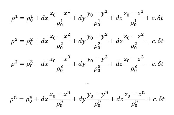
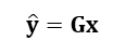
The set of equations above can be re-written in matrix form as:
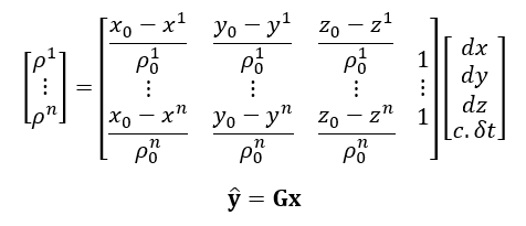
Where G is called as the design or geometry matrix of navigation equations.
From the equation above, to have an averaging effect to reduce random error, the equation should be overdetermined, that is, $n \geq 4$.
Hence, the solution of x can be solved as:
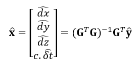
And the estimated location of a receiver X is:
The equation above will be calculated (solved) iteratively for few iterations until the estimated $\hat{x}$, the estimated $dx,dy,dz$, is converge to some small values.
For standard GNSS position calculation, after few iterations, the solution will converge with initial location guess at the centre of the earth.
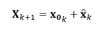
In each iteration step $k$, the receiver location will be updated as:
Error and Variance analysis
Further error (residuals) and variance analysis can be evaluated from the navigation equation:
The residual (post-fit) of the fitting or estimation process can be calculated as:
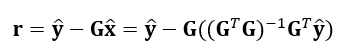
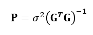
Assuming uncorrelated values (data), the covariance matrix obtained from the navigation equation can be calculated as:
READ MORE: Measurement uncertainty estimations: GUM method
Uncertainty contributors from linearised navigation equation
To determine the uncertainty contributors of GNSS position measurements, we can derive the contributors from the measurement equation, that is the set of navigation equations.
From the set of navigation equations, we can observe three main factors affecting the GNSS positioning calculations.
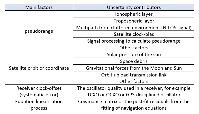
The three main factors are:
- Pseudorange.
As the pseudorange is calculated from the multiplication of the time of flight of a GNSS signal (from a satellite to a receiver) and speed of light, we can directly spot that, since the speed of light is usually fixed at a known value, the time of flight is affected by manufacturers.
These factors can either delay or advance the signal while travelling to a receiver.
Several main factors that significantly affect GNSS signal time of flight [1,2] are:
- The thickness of ionospheric layer. This layer can cause delay of GNSS signals (electromagnetic wave) and also advance the phase of the signals. This delay can significantly introduces errors on a true pseudorange value. The delay due to ionospheric layer can be modelled by Klobuchar (GPS) and NeQuick model (GALILEO) [1,2,3].
- The thickness of the tropospheric layer. This layer can also cause some delay on the GNSS signal time of flight (travel time). The delay introduces by this layer when a GNSS signal enter the earth, has a higher variation than the delay introduced in the ionospheric model.
- Multipath from environment. Urban or city environment are usually cluttered and cause GNSS signal to be deflected, re-bounced such that multipath impairments are introduced on the signal. These multipaths cause delays on the arrival time of the GNSS signal to a receiver compared to straight line-of-sight signal travel path.
- Satellite clock-bias. When the travel time (time of flight) of a GNSS signal has been estimated, besides delay introduced by the previous factors, there is also an effect from the bias of the clock that is on-board on a GNSS satellite. This satellite clock-bias can cause the calculated pseudorange to be shorter or longer depending on the clock-bias.
- Signal processing to calculate a pseudorange. The calculation of pseudorange is highly related to the algorithm used to process the receive GNSS signal. This algorithm needs to locate the first sample of the ranging signal (GNSS signal) that arrives at the receiver and estimate the time to reach the preamble of the signal by considering an estimated actual PRN code length in 1s (code frequency) per 1s epoch [1,2].
- And other factors.
- Satellite orbit or coordinate.
To calculate satellite’s $x,y,z$-coordinates or orbits when the satellite transmit a processed GNSS signal, broadcasted ephemeris inside the satellite GNSS signal should be demodulated. This ephemeris provides values and constants to calculate the satellite orbit location.
However, there will be errors between the estimated satellite orbit and the actual satellite orbit. Because, space disturbances will affect the dynamic of a satellite and hence cause a displacement of the satellite with respect to its planned orbit path [5].
The space disturbances can be from the solar pressure of the Sun, space debris and gravitational forces from the Moon and the Sun and other factors.
Also, the orbit (including the algorithm used to estimate the orbit) upload link from the master ground station to a GNSS satellite also affects the correctness of the satellite orbit or coordinate.
- Receiver clock-offset (systematic error).
Receiver clock-offset is the difference between the receiver clock and the GNSS system time. it is well-known that the clock quality of the receiver is far lower than the clock quality of an on-board satellite clock.
For example, the clock on a receiver drifts much faster than the satellite clock drift.
However, this receiver cock-offset is systematic and can be estimated by solving the navigation equations.
One important think to note is that it is assumed that all the GNSS signal sampled at the same time (clock) at a receiver.
- Other effects, such as the linearisation of the navigation equations.
The linearisation of a set of navigation equation introduces some errors on the calculation of positions from GNSS signals.
These errors introduce uncertainty on GNSS position measurements due to the linearisation processes by applying Taylor-series approximation.
The uncertainty due to this linearisation process can be estimated from the covariance matrix calculated from the linearised navigation equations or from the post-fit residual calculations.
Table 1 provide the summary list of possible uncertainty contributors that can be derived from the high-level set of navigation equations. This list of uncertainty contributors is derived from the main factors affecting the GNSS position calculation from a set of navigation equations.
Final note is that since the set of navigation equations are complex, a linearisation process and iterative algorithm need to be applied to derive a position.
From the previous post (Part 1), to estimate measurement uncertainty, the reference method is the GUM method. However, since we have a complex set of navigation equations, we can resort to an alternative method, such as spreadsheet method or Monte-Carlo simulation method to estimate the uncertainty.
The above list of uncertainty contributors will be used to estimate the uncertainty with the spreadsheet or Monte-Carlo simulation method.
READ MORE: Correlator outputs for clean and spoofed GPS L1 C/A signals
Conclusion
In this post, we have discussed about the formation of navigation equations and how to solve the equations by using a linearisation and iterative algorithm.
The main results of solving the navigation equations are to get the estimate of the position of a GNSS receiver as well as the clock-bias of the receiver.
There two important elements in the navigation equations: pseudorange and satellite location (the receiver-clock bias is the by-product estimate from solving the navigation equations as this is a systematic error).
Hence, many factors affecting the pseudorange calculations and satellite locations, these factors are directly considered as relevant uncertainty contributors calculated GNSS positions.
From the navigation equation, we can derive the uncertainty contributors on GNSS position measurements from those main affecting factors.
Reference
[1] Kaplan, E.D. and Hegarty, C. eds., 2017. Understanding GPS/GNSS: principles and applications. Artech house.
[2] P. Misra and P. Enge. 2006. “Global Positioning System: Signals, Measurement and Performance.” 2nd edition.
[3] J. S. Subirana, J. M. J. Zorboza, M. Hernandez-Pajarez (2013). GNSS data processing. Volume 1: Fundamentals and algorithm. European Space Agency (ESA).
[4] F. Van Diggelen. 2009. “A-GPS: Assisted GPS, GNSS, SBAS”.
[5] Syam, W.P., Priyadarshi, S., Roqué, A.A.G., Conesa, A.P., Buscarlet, G. and Orso, M.D., 2023, September. Transformer deep learning for accurate orbit corrections in real-time. In Proceedings of the 36th International Technical Meeting of the Satellite Division of The Institute of Navigation (ION GNSS+ 2023) (pp. 159-174).
You may find some interesting items by shopping here.