Data forecasting: The difference with interpolation and a practical example
Data forecasting or extrapolation is rudimentary different with data interpolation. In this post, we will explain the difference between forecasting (extrapolation) and interpolation in a simple manner and with a practical example.
Data forecasting or extrapolation is rudimentary different with data interpolation. In this post, we will explain the difference between forecasting (extrapolation) and interpolation in a simple manner and with a practical example.
Data forecasting (extrapolation) is a type of time-series analysis where we want to predict future observations from previous observations.
These previous observations are sequential with constant time-step. That is why we call it as time series data.
Many useful applications for data forecasting includes predicting future product demands for logistic planning, predicting future stock prices and predicting future weather patterns.
Methods for data forecasting are also cardinally different with those for data interpolations (examples of data interpolation include such as regression and classification).
By the end for this post, we will understand the fundamental different between data forecasting (interpolation) and data interpolation (such as regression and classification).
Let’s go into the discussions and example.
Interpolation vs extrapolation
Very often, we can find people mistakenly understand that interpolation and data extrapolation (forecasting) are identical. However, these two data estimation processes are completely different.
In this section we will discuss the fundamental differences between interpolation and extrapolation (forecasting).
Interpolation
Data interpolation is a process to estimate a new output data from a given input data based on an estimated function from previously observed input-output pairs.
In mathematical formulation, data interpolation is constructing a function that maps inputs $x$ to output values $y=f(x)$ and is modelled as:
Where $f(x)$ is a learned or fitted function obtained from previously observed $x$ as input and $y$ as output pairs.
An important property of interpolation is that the output estimation is designed to be within the range of existing ranges of previously observed data. Otherwise, interpolation will give an estimation with large error.
In interpolation, the sequence and constant space of data is not essential.
The main applications for data interpolation are regression and classification problems.
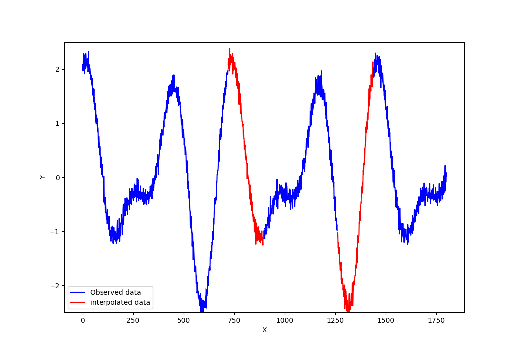
Figure 1 below shows and example data interpolation of a periodical function. In figure 1, the previously observed data are in blue and the interpolated data are in red.
We can observe that the interpolated data is within the range (minimum and maximum) of the previously observed data.
Extrapolation (forecasting)
Data extrapolation (forecasting) is a process to estimate new outputs from using the previous sequence and equally-spaced of output values [1,2].
Data extrapolation estimates outputs that are outside the range of previous observed outputs.
In mathematical formulation, data extrapolation is building a function that maps sequential and equally spaced in time previous observation $y_{prev}$ to sequential and equally-spaced in time future observation $y_{next}$ as follows:
Where $f(y_{prev})$ is an estimated function from previous sequence of output data with equally spaced in time.
Unlike regression analysis, from this equation, time series models for data extrapolation or forecasting have dependent variables which are a function of past values of the dependent variable themselves [3].
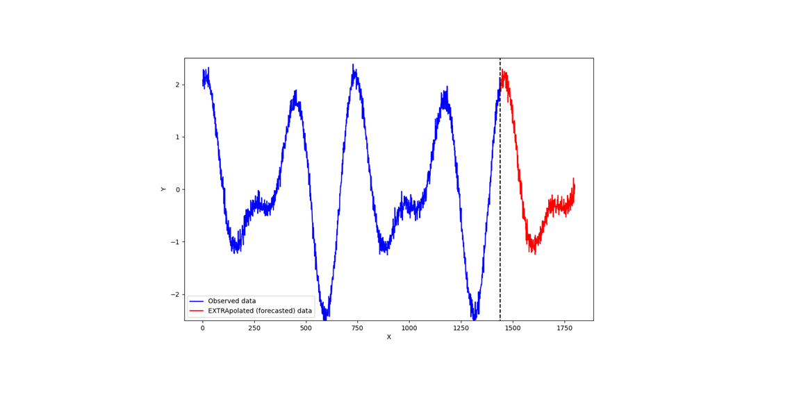
Figure 2 below shows the illustration of data extrapolation. In this case, the extrapolated (forecasted) data are outside the range of the previously observed data.
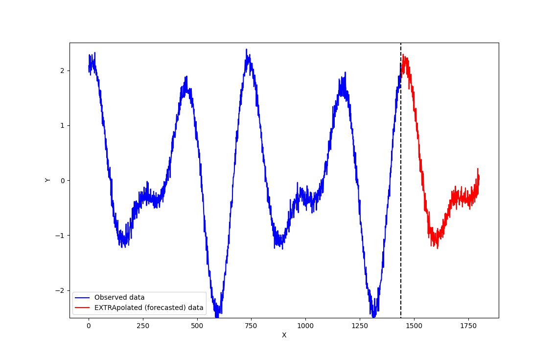
That is, data extrapolation is commonly known as time series analysis.
An important property of time series analysis is the model operates on a sequence of data of successive equally spaced points in time.
An example of a well-known statistical time series model is moving average, autoregressive and ARIMA [3].
Four main variational characteristics of time series model for data extrapolation are as follows [3]:
- Seasonal variations that is repeating over a specific period such as a day, week and month,
- Trend variations that is as long-term increase or decrease in the data, either linear or non-linear,
- Cyclical variations that is exhibiting rises and falls that are not of fixed period
- Random variations that are other than the three variation types.
These four different types of variations sources in data for time series modelling cause numerous challenges to produce an accurate time-series data forecasting [3].
One important aspect we need to put attention on time series modelling for data extrapolation is our time series data should not follow a random walk process [4]. Because no model can predict a random walk process or univariate Brownian motion time series data.
In a random walk process data, the next time step output will be a function of the prior time step observation [4]. Because random-walk process has characteristics of strong temporal dependence (autocorrelation) that decays linearly [4].
One way to validate or check a time-series data as a non-random walk process are by:
- Analysing the autocorrelation function and specific tests like the Augmented Dickey-Fuller test [3] or,
- Plotting the time series prediction and ensure the prediction is not the output of the prior time step [4].
Practical example of extrapolation problem
Traditionally, time series modelling use purely statistical method to model future data from previously time-sequenced data observations, such as ARIMA [1].
A fundamental assumption of purely statistical time series models are [1,2,3] data sequences should be stationary, meaning the mean and variance of the time series data should be constant over time (independent with respect to the time location, but only depends on time length) and there is no seasonality.
In this practical example, we use machine learning model to learn previously time series data to predict future time series data.
With machine learning, we can perform interpolation (such as regression and classification) or extrapolation or forecasting (such as time series or sequential data analysis), depending on how we arrange input-output and select a model [5].
In this demonstration, we will use python to implement the data extrapolation with a simple neural network model.
We will demonstrate the data extrapolation case study by learning a simple periodical function as follows:
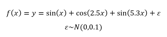
Data input and output as follows:
input_length=360*3
output_length=360

n_train=600
n_test=50
From the input and output data, we use input data of the length of three periods or cycles (360*3) and we want to predict output for the next one period or cycle. The reason of using three cycles of data input is to make sure that our input data capture all-time series variation sources: seasonality, trend and cyclical (as have been explained above).
Data generation in Python is as follows:
n=360*1000
x=np.linspace(1,n,n)

y=np.sin(x*3.14/180)+np.cos(x*3.14/180)+np.cos(2.5*x*3.14/180)+np.sin(5.3*x*3.14/180)+np.random.randn(n)*0.1 #TYPE 3

x=np.matrix(x)
y=np.matrix(y)

x2_train=np.zeros((n_train,input_length,input_dim),dtype=float)
x2_test=np.zeros((n_test,input_length,input_dim),dtype=float)

x_train=np.zeros((n_train,input_length,input_dim),dtype=float)
y_train=np.zeros((n_train,output_length),dtype=float)

for ii in range(n_train):
    temp=y[0,ii:ii+input_length]
    temp=np.repeat(temp,input_dim,0)
    x_train[ii,:,:]=np.transpose(temp)
    y_train[ii,:]=y[0,ii+input_length:ii+input_length+output_length]

x_test=np.zeros((n_test,input_length,input_dim),dtype=float)
y_test=np.zeros((n_test,output_length),dtype=float)

for ii in range(n_test):
    temp=y[0,ii*(n_train+1):ii*(n_train+1)+input_length]
    temp=np.repeat(temp,input_dim,0)
    x_test[ii,:,:]=np.transpose(temp)
    y_test[ii,:]=y[0,ii*(n_train+1)+input_length:ii*(n_train+1)+input_length+output_length]
Since the function is periodical every 360 degree, we generate 1000 periodic data. From these 1000 periodic data, we separate them for training and test (in this case for model validation) set.
The simple neural network model is as follows:
class TimeSeriesModel(nn.Module):
    def __init__(self, input_length,output_length,input_dim,d_model,nhead,num_layer):
        super().__init__()

        self.input_length=input_length
        self.output_length=output_length
        self.d_model=self.input_length

        self.flatten = nn.Flatten()
        self.mlp1=nn.Linear(self.input_length, self.d_model)
        self.mlp2=nn.Linear(self.d_model, self.output_length)

    def forward(self,x):
        x = self.flatten(x)
        x = self.mlp1(x)
        out=self.mlp2(x)

        return out
We only use a simple neural network with only one hidden layer because the model to learn is also very simple.
The training and test (in this case for model validation) processes are as follows:
optimizer = Adam(transformer.parameters(), lr=0.0001) #lr=0.001
criterion = nn.MSELoss() #loss function for regression

for epoch in range(epochs):

    """#Training"""
        transformer.train()

    training_loss = 0.0
    for i, data in enumerate(train_loader, 0):
        inputs, labels = data
        inputs, labels = inputs.to(device), labels.to(device)

        optimizer.zero_grad()

        outputs = TimeSeries(inputs)


        loss = criterion(outputs, labels)
        loss.backward()
        optimizer.step()

        training_loss += loss.item()

    print(f'Epoch {epoch + 1}/{epochs} Training loss: {training_loss  / len(train_loader) :.3f}')


    """# Testing"""

    TimeSeries.eval()

    test_loss = 0.0
    with torch.no_grad():
      for data in test_loader:
        input, labels = data
        input, labels = input.to(device), labels.to(device)

        outputs = TimeSeries (input)

        loss = criterion(outputs, labels)
        test_loss += loss.item()

      print(f'Epoch {epoch + 1}/{epochs} Test loss: {test_loss  / len(test_loader) :.3f}')


    if(test_loss<0.05 or training_loss<0.05):
        break
For training, we use the standard Adam optimiser and mean square error loss function.
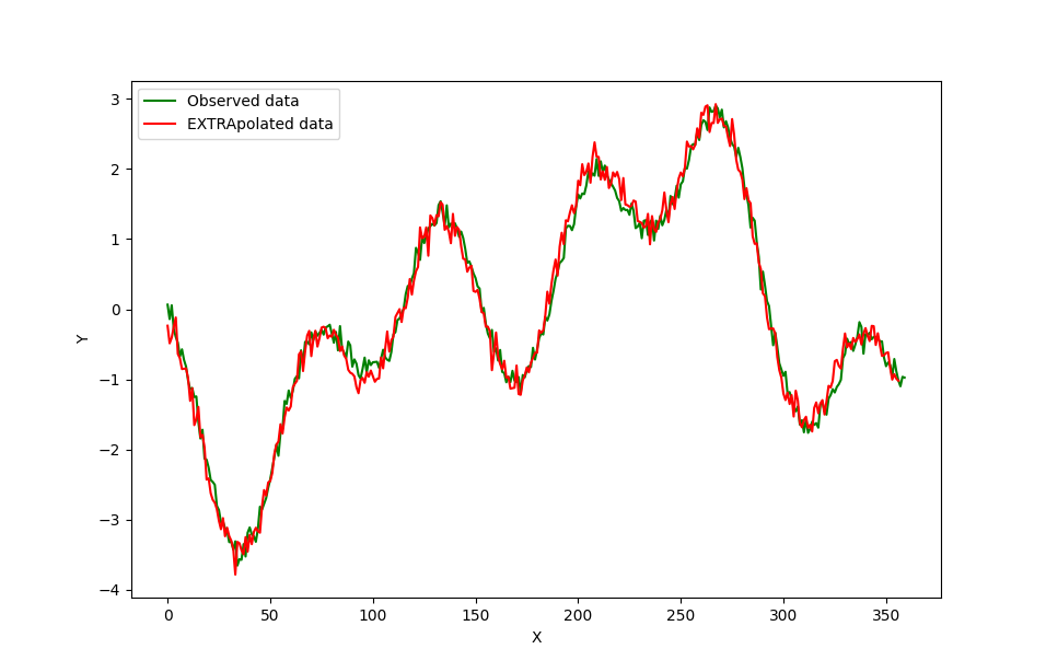
The results of the data extrapolation compared with the ground truth is shown in figure 3 below. As we can see, the extrapolated data in red agree with the ground truth in green.
From figure 3, the neural network also learn the high frequency noise in the data (the random noise). We can apply a low pass filter to smooth the data.
The process of the data extrapolation is shown in a vide below:
READ MORE: US vs UK-EU economy: How US economy grows much bigger and faster than UK-EU economy
Conclusion
In this post, we have discussed the fundamental difference between data interpolation and data extrapolation (forecasting). In data extrapolation, we focus on predicting outputs from previously equally time-spaced sequence outputs.
That is, we are interested in building a function that maps previous output to future outputs instead of mapping and input to output as in the case of interpolation.
To make data extrapolation clearer, we demonstrate a data extrapolation case study with a simple neural network model.
From here, readers can differentiate between data interpolation and extrapolation so that correct methods can be chosen to solve either problem.
Reference
[1] Cryer, J.D., 2008. Time series analysis. Springer.
[2] Shumway, R.H., Stoffer, D.S. and Stoffer, D.S., 2000. Time series analysis and its applications (Vol. 3, p. 4). New York: springer.
[3] Hamilton, J. D. (2020). Time series analysis. Princeton university press.
[4] Durlauf, S. N., & Phillips, P. C. (1988). Trends versus random walks in time series analysis. Econometrica: Journal of the Econometric Society, 1333-1354.
[5] Goodfellow, I., Bengio, Y., & Courville, A. (2016). Deep learning. MIT press.
You may find some interesting items by shopping here.