Predicting the cost directly when allocating the tolerance of the key characteristic (KC) of a mechanical assembly

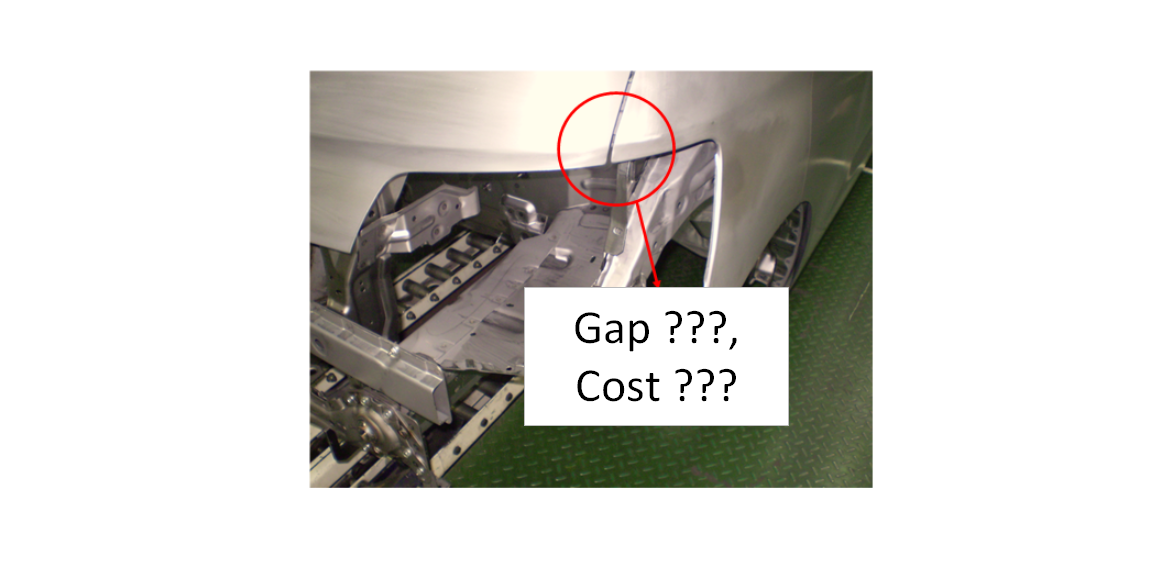
In a car factory, when they want to change the gap between an engine hood and side fender within few or less mm, this change will cost thousands or even much more of dollars to the factory.

Similarly, if a gearbox factory wants to change their design of the distance between two axes just few or less mm, they will spend a lot of dollars to make that change.

The reason is that a small change on the key characteristics (KC) or functional requirement of an assembly will affect all parts and their features tolerance allocations involved in the gearbox assembly chain.

Allocated tolerance values on the features of each part will have significant economic impact on the manufacturing cost, such as more machining time, more precise machining requirements, and/or new assembly sequences and fixturing systems.

This post discusses a direct estimation of cost when we determine or change the KC of an assembly.

Having said that, this post is only a brief explanation of estimating the cost of assembly requirements (that is the KC) directly from the KC’s allocated tolerances summarised from the paper of Prof. Armillotta (Politecnico di Milano) in reference [1] and [2].

In addition, this post cannot do justice in thoroughly explaining the paper in detail. So, we recommend reading the paper by reader themselves to get the comprehensive understanding of the cost estimation of the KC of mechanical assemblies.

Do you want to have good research philosophies and improve your research management and productivity?

This book is a humble effort to map well-known and proven principles and rules from various disciplines, such as management, organization decision theory, leadership, strategy, finance and marketing, into a single practical research guide that applies to all disciplines.

You can also get this book from Rakuten Kobo.

Tolerance allocation for assembly key characteristic (KC)

Tolerance allocation is an activity to assign tolerance values on the feature of a part after the tolerance types (dimensional and/or geometrical tolerance) have been determined.

The main purpose of tolerance allocation is to determine the tolerance value of all features in an assembly chain such that the KC of the assembly is satisfied.

For example, the gap between the fender and engine hood of a car should be $2mm \pm 0.1 mm$.

In ideal situation, the KC of an assembly is defined as:

Where is $Y$ the KC or functional requirement of a mechanical assembly, $X_{0_i}$ is the nominal or expected value of feature $i-th$ constituting the KC and $T_{Y}$ is the allowed variation (tolerance) of the KC to satisfy the specific requirement or functionality of a mechanical assembly.

It is important to note that we cannot directly control the value $Y$ (the KC). Because the values of parts constituting the assembly KC $Y$ determine the final value of the KC $Y$.

This is called “tolerance variation stack-up”, that is the variation of parts will stack and accumulate until the final dimension $Y$ (the KC).

In reality, variations occur due to machining and assembly errors.

Hence the KC $Y$ becomes:

Where $S_{i}$ is a variable that describe how sensitive $Y$ with respect to feature $X_{i}$. Often, we assume $S_{i}=1$, meaning all feature dimensions in the KC’s tolerance chain are equal in term of affecting the $Y$.

Meanwhile, $X_{i}$ is the $i-th$ dimension that is vary due to process errors (such as machining, assembly, stamping and other processes).

Hence, $X_{i}$ is modelled as:

Where $T_{i}$ is the tolerance of $X_{0_i}$.

Meanwhile $T_{Y}$ is statistically calculated as:

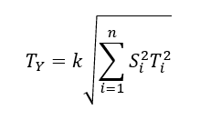
That is, $T_{Y}$ is the total tolerance stack-up from feature tolerances constituting the assembly and $k$ is a “safety factor” to take additional (not quantified) part variations contributed from other suppliers.

When we change the KC of an assembly, this change will massively impact the total manufacturing and assembly cost of the assembly [1,2].

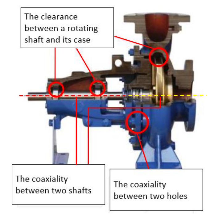
For example, in figure 1 below, a centrifugal pump assembly can have many KCs or assembly requirements.

In figure 1, at least there are four KCs on the assembly, they are the alignment of the two axes of a shaft and pump, the coaxiallity of the holes, and several clearance requirements.

A small change in these KCs dimensions will affect how each part in the assembly chain will be finish machined or how all the parts should be assembled together (maybe it requires a fixture modification on the assembly processes).

Tolerance optimisation

To assign tolerances on features on an assembly, the easiest way is by using heuristics and intuitions by adjusting the tolerance values and try to estimate the total variation such that the variation is still within the allowed variations $T_{Y}$ in equation (4).

However, this heuristic way may not consider the effect of changing the value of feature tolerances on the total manufacturing and assembly cost.

A better way in allocating tolerance is by solving an optimisation problem. The optimisation problem is to minimise the total cost while still satisfying the allowed assembly variation $T_{Y}$ as modelled in equation (5) below.

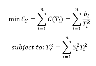
Where $C_{Y}$ is the total assembly and manufacturing cost, $C(T_{}i)$ is the tolerance cost of the $i-th$ feature dimension $X_{i}$ and $T_{i}$ is the assigned/allocated tolerance for the feature dimension $X_{i}$.

The tolerance cost is a function of tolerance vs cost, mostly the machining process cost of the corresponding features.

Note that the smaller the $T_{Y}$, the smaller the allocated tolerance for $T_{i}$, the higher the manufacturing and inspection cost (small tolerances will require a high accurate measuring instrument).

The formula to calculate $b_{i}$ and the value of exponent $k=0.55$ is determined in [3].

$b_{i}$ is formulated as:

Where:

• $\beta =0.4 \times 10^{-3}$,
• $f_{Mi}$ is a coefficient depending on feature materials, such as steel, aluminium or titanium. The harder the material, the higher the machining cost will be,
• $f_{Fi}$ is a coefficient depending on feature types, such as hole, shaft, slot or curve surface. The more complex the feature the higher the manufacturing cost will be,
• $f_{Ai}$ is a coefficient depending on feature area (in $cm^{2}$). This feature area will directly affect the machining time.

The values of $f_{Mi}$ and $f_{Fi}$ are obtained by historical data from manufacturing industries.

From the tolerance optimisation model shown in equation (5) above, equation (4) becomes the constraint of the optimisation function where a total cost should be minimised.

However, there is a problem though with this tolerance optimisation to minimise the cost of a mechanical assembly.

There is variable $T_{i}$ that is the allocated tolerance for each feature dimension $X_{i}$. Meaning, we need to solve the optimisation problem which is not easy.

It is not easy to solve the tolerance optimisation problem with a non-linear function and constraint. Solving this optimisation will require an iterative or heuristic algorithms and may not be practical in industries.

This difficulty of solving the tolerance optimisation reduces the practicality of the tolerance optimisation for industry to use.

Hence, to make this cost minimisation problem more practical than solving the optimisation problem, a way has been proposed in [1], that is to estimate the assembly cost $C_{Y}$ in equation (5) without the need to solve the optimisation problem.

READ MORE: 2D tolerance stack-up analysis with examples

Estimating cost directly from the KC of an assembly without solving the tolerance allocation problem

As allocating tolerances is not an easy task, especially when the assembly chain involves many features, we need a way to estimate the total assembly and manufacturing cost $C_{Y}$ to satisfy the KC of a mechanical assembly directly from the allocated KC’s tolerance $T_{Y}$.

This direct cost estimation $C_{Y}$ is central in this blog discussion. Prof. Armillotta in his paper [2] proposes a way to directly link the cost $C_{Y}$ of a mechanical assembly to its KC tolerance $T_{Y}$ utilising the Lagrange multiplier method [1].

The proposed model directly estimate the assembly and manufacturing cost $C_{Y}$ as a function of $T_{Y}$ so that we do not need to solve tolerance allocation problems to assign value to each feature tolerance $T_{i}$.

The proposed closed-form mathematical model of $C_{Y}$ as a function of $T_{Y}$, is:

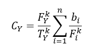
Where $k=0.55$, $b_{i}$ is calculated as in equation (6) above, and $F_{i}$ and $F_{Y}$ are calculated as:

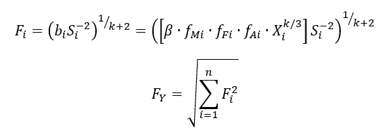
Where $F_{i} \sim T_{i}$ is called “optimal scaling factor” and $S_{i}$ is the sensitivity of the KC dimension $Y$ with respect to $i-th$ feature $X_{i}$.

As we can observe from the above model, we can directly relate $C_{Y}$ as a function of $T_{Y}$ and hence we do not need to solve tolerance allocations for $T_{i}$ of each feature dimension $X_{i}$.

That is, with this new model in equation (7), we can directly estimate the cost of a mechanical assembly with KC dimension $Y$ with desired tolerance of $T_{Y}$.

For example, from figure 1 above, when we want to set the alignment tolerance (coxiallity) between the axis of the shaft and centrifugal motor on figure 1, we can estimate how much the total cost will be considering the machining process, feature type and size for each feature involved in the assembly chain.

In [1], there are several excellent examples on the use of the new cost model to estimate the cost of the tolerance of KCs (functional requirements) of various mechanical assembles.

READ MORE: Examples on how to interpret GD&T: Form, orientation, location and run-out tolerances

Does performing tolerance optimisation to determine assembly cost worth it?

Now, another question emerges. How beneficial the use of the cost model and the “optimal scaling factor” $F_{i}$ in equation (7) is compared to commonly and established “scaling factors” to estimate $F_{i}$ and then the total assembly cost of the KC of a mechanical assembly.

There are several established and commonly used scaling factors that are [2]:

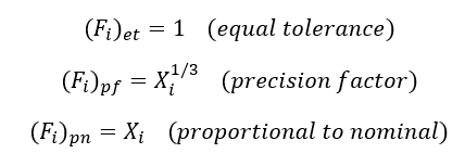
Meanwhile, the proposed $F_{i}$ in [1], calculated by equation (8) above, is obtained by solving the tolerance optimisation problem in equation (5) above by using Lagrange multipliers.

If we compared this “optimal scaling factor” $F_{i}$ in equation (7) to the establishes scaling factors (in equation (9) above): equal tolerance, precision factor and proportional to nominal, the “optimal scaling factors” seems to be much more complicated and requires more data.

We can see that the “optimal scaling factor” $F_{i}$ in equation (7) also considers the material, geometry and size of features $X_{i}$.

The question is whether it is worth it to use the more complex “optimal scaling factor” compared to the three “established scaling factor”.

The answer is yes and depends in two situations [2]:

• In the case that all parts in an assembly use the same materials and similar shape and size, the “optimal scaling factor” will give optimal allocation but the benefit over the three traditional and established scaling factors (equation (9)) is not by significant margin.

Because, if the materials are the same and the size and geometry are similar, the difference in manufacturing cost usually only on the finishing process.

• However, if the parts in an assembly consist of very different materials, different size and geometry, the benefit of using “optimal scaling factor”, compared to the three established scaling factors, is huge.

READ MORE: 3D tolerance stack-up analysis with examples

Conclusion

In this post, we have discussed a way to directly estimate the total cost of a mechanical assembly given a certain functional requirement (KC) to satisfy.

For example, the assembly of a centrifugal pump requires the coaxiallity between the axis of the shaft and pump should be within a specific tolerance.

This post presents a brief reminder of a tolerance stack up and how to statistically calculate the total tolerance stack up from the tolerance of its features as well as tolerance optimisation function (which is not easy to solve) to minimise the total cost of mechanical assemblies.

Based on [1] proposed by Prof. Armillotta, this post then discusses the model on how to directly estimate the assembly cost without solving the tolerance allocation problem. Instead, we can directly estimate the assembly cost from its given value of KC.

Finally, this post also presents the benefit of using the “optimal scaling factor” presented in [2] compared to three previously common “scaling factor”.

References

[1] Armillotta, A., 2023. Estimating the cost of functional requirements for tolerance allocation on mechanical assemblies. The International Journal of Advanced Manufacturing Technology, 129(7), pp.3695-3711.

[2] Armillotta, A., 2024. Estimation of cost reduction by tolerance optimization. The International Journal of Advanced Manufacturing Technology, 134(3), pp.1379-1393.

[3] Armillotta, A., 2022. An extended form of the reciprocal-power function for tolerance allocation. The International Journal of Advanced Manufacturing Technology, 119(11), pp.8091-8104.

You may find some interesting items by shopping here.