GNSS

TUTORIAL on how to measure RF receiver noise: A practical approach

In this post, we will provide tutorial on how to quantify a receiver (instrument) noise. In addition, the basics of various unit of measurements related to signal processing will be discussed.

Wahyudin Syam

Jul 31, 2024 • 10 min read

In signal processing, the noise from a radio frequency (RF) signal receiver significantly affects the quality of the processed signal and hence is influential to the performance of a signal processing algorithm.

In this post, we will provide tutorial on how to quantify a receiver (instrument) noise. In addition, the basics of various unit of measurements related to signal processing will be discussed.

With respect to the basics of the unit related to signal processing, there are different units: dB, dBm, dBW, dB/Hz, dB-Hz and other units.

These units may be confusing for many people. We will clarify the different of these units in this post.

By the end of this post, we will understand the basics of power and noise measurement including their relevant units and the practical procedure to quantify the noise of an RF receiver.

Do you want to have good research philosophies and improve your research management and productivity?

This book is a humble effort to map well-known and proven principles and rules from various disciplines, such as management, organization decision theory, leadership, strategy, finance and marketing, into a single practical research guide that applies to all disciplines.

The book’s chapters cover: How do you determine the primary research tools? How do you select research philosophies? How do you make research strategies? How do you determine research innovation? How do you navigate complex research? How do you economically justify research? How do you economically value research? How do you manage research? How do you market research?

You can also get this book from Rakuten Kobo.

Revisiting the basics of signal and noise measurement unit

Let’s us revisit the basics of signal and noise power measurements. People who already familiar with this concept may skip this section. But we think there are still many people who need to understand these foundational concepts.

dB and dBm

Let’s us start from the very basics question, what is the difference between dB and dBm?

Yes, there are still many people that are still not correctly understand the different between dB and dBm.

The difference between dB and dBm are:

dB is a constant and dBm is a measured quantity.

dBm or dBW is a unit of measured power. We require a physical power measurement sensor or device to measure the value of a signal’s power.

A signal generator and power spectrum analyser have an embedded sensor to measure the power of a signal.

Meanwhile, all signals after being received from a receiver will be converted into numbers (which has a range that depends on the number of bit resolution of the analog-to-digital/ADC in the receiver, e.g. 16-bit, 32-bit or 8-bit. Since the signal that we process is only numbers, all calculations are only in dB since we do not know anymore what the actual received signal power was.

dB is the 10*log(“number”) and is only a constant transformed to dB scale. Meanwhile, dBm or dBmW is the 10*log(“a measured power quantity”) in mW or W respectively. dBm can be converted to dbW by subtracting 30 from the dBm value. Otherwise dBW can be converted into dBm by adding 30 from the dBW value.

For example, $0dBW = 30dBm$, $1dBW = 31dBm$, $0dBm = -30dBW$ and $1dBW = -29dBm$.

dB can be “added” or “subtracted” with either another dB constant or another dBm or another dBW quantity. Meanwhile, dBm can only be “added” or “subtracted” with dB or dBm only and not with dBW (unless the unit has been equalised in either mW or W).

Because it is a constant, dB can be “added” or “subtracted” (equal to a “multiplication operation” or “division” in non-dB scale, respectively) with either another constant in dB or another measured quantity, e.g., in dBm. But not otherwise.

Remember, addition and subtraction operation in dB scale are equal to “multiplication” and “division” in normal scale.

For example, $30dBm+5dB = 35dBm$, $45dBW-20dB = 25dBW$ and $25dBm+5dBm=30dBm$. But we cannot do $30dBW+15dBm$.

dB, dB-Hz and dB/Hz

There are three main types of dB unit that always come together in signal processing: dB, dB-Hz and dB/Hz (or dBm, dBm-Hz and dBm/Hz).

dB (or dBm in case we know the signal power by measurement).

dB is obtained by taking calculations of 10log of the square of the amplitude of a signal in time domain. This is straight forward and already well-known.

dB/Hz (or dBm/Hz in case we know the signal power by measurement).

The noise density $N_{0}$ (remember, it is different with noise $N$) of a signal is represented in $dB/Hz$ (or $dBm/Hz$ is the actual signal power is known). Because a noise of signal is limited by frequency (bandwidth), that is noise is defined per frequency bin, that is, noise per unit Hertz.

Noise should be defined over a specific frequency bandwidth (per frequency bin-width in a signal spectrum or $/Hz$).

An important note, judging a signal noise only by observing the spectrum of a signal can be misleading if not done carefully. Because, the more frequency bins used in the spectrum, the lower the noise will be since the noise power is distributed into more bins.

dB-Hz (or dBm-Hz in case we know the signal power by measurement).

dB-Hz is the unit for C/N0 (note that C/N0 and SNR are different). This is the measure of the signal power with respect to the signal noise. Meanwhile, the unit of SNR is dB since it is the ratio between signal power (in dB or dBm) and noise (also in dB or dBm).

In short, noise density is $N_{0}$ (dB/Hz or dBm/Hz) and signal noise is $N$ (dB or dBm).

Since this value is obtained by dividing a signal power with its noise (where noise is defined as $/Hz$). The C/N0 unit will be $unit-Hz$ or if it is scaled it will be $dB-Hz$.

Figure 1 below illustrate dB, dB-Hz and dB/Hz from a calculated spectrum of a signal (in frequency domain). In this figure, the dB is the summation of the signal power (converted from the spectrum value) over several frequency bins, dB/Hz is the spectrum value per each bin and dB-Hz is the difference between dB (signal power) and dB/Hz (noise floor).

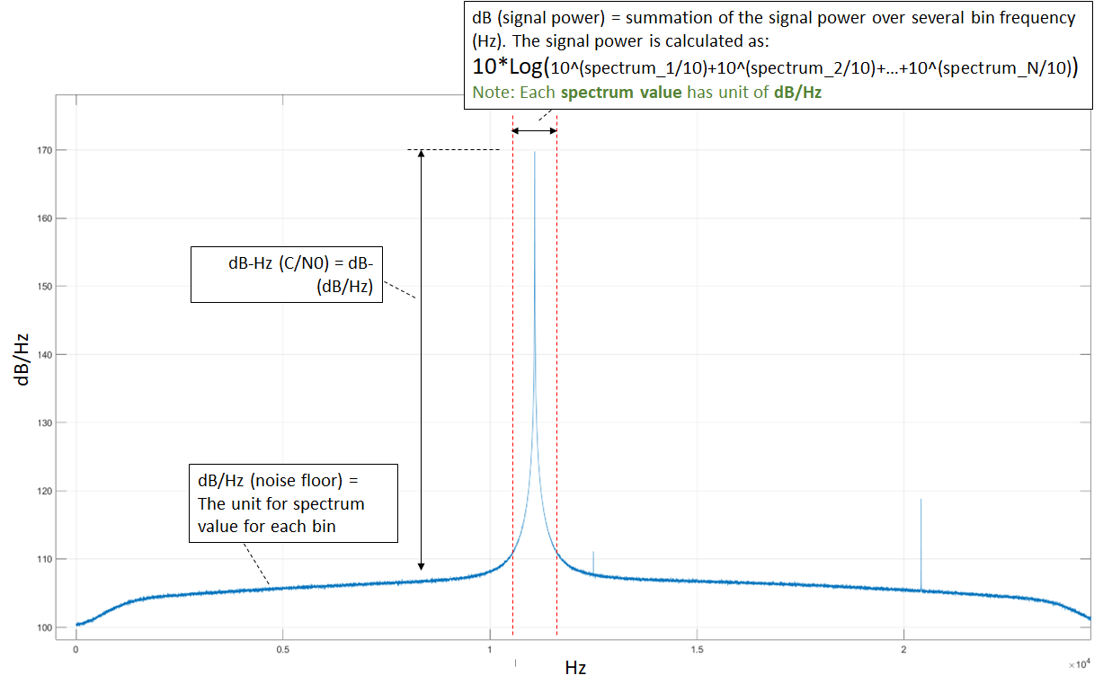
Figure 1: The illustration of dB, dB-Hz and dB/Hz in a signal spectrum.

To summary, when we process a signal received by a receiver, all calculations will be in dB, dB-Hz or dB/Hz for signal power, C/N0 or noise density or noise per unit Hertz, respectively. Because, at this point, we do not know the actual power of the signal when the signal is received.

The signal that we process is only a sequence of number (we lost the knowledge of the signal’s actual power), depending on the resolution of the bit of the receiver, it can be a number between -32768 to 32767 for 16-bit integer or other value limits.

We do not know the power (in mW or W) of the signal anymore. The power of a signal can only be quantified by performing a power measurement procedure using a specific physical sensor.

If we generate a signal using a signal generator or signal simulator hardware, or if we capture a signal with a spectrum analyser, there will be a power measurement sensor inside these instruments so that we can know the power (commonly in mW or W) of the signal.

In this case, when we know the power unit, our calculation results will be in dBm or dBm-Hz or dBm/Hz.

RF receiver noise estimation procedure

A perfect electronic device with zero noise will have noise power (noise floor) for $10log(0)=- \inf$. Hence, the less perfect the electronic device the higher the noise (noise floor) it will get. That is the noise floor will raise from the ideal value of $-\inf$ to some value (typically to some minus hundreds).

The point is the lower the noise floor, the better the receiver sensitivity. Because a low noise floor means there is high probability a signal can be received above the noise floor and can be processed properly.

The next section, we will discuss the setup and procedures for receiver noise estimation.

The setup

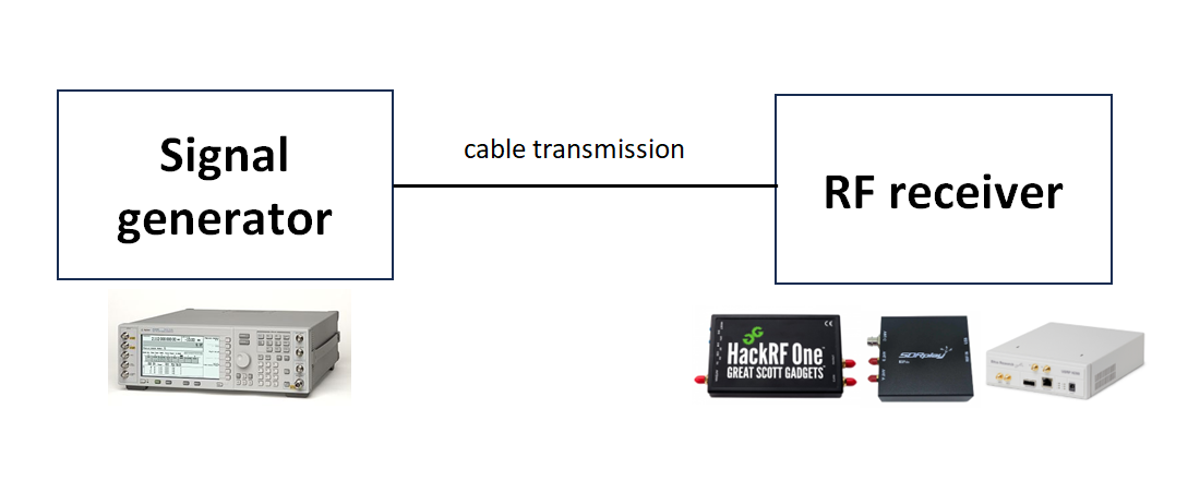
The setup used to estimate RF receiver noise is shown in figure 2 below. In this figure 2, the setup is not complex and is straightforward.

We need only three components:

A signal generator.

The signal generator is used to know the transmit power (typically in dBm) and to generate a known signal, typically a sine tone signal at specific sampling frequency.

A receiver under test.

The receiver under test is the RF receiver that we want to estimate the noise.

A cable for signal transmission.

This cable is used to transmit the signal from the signal generator to the receiver under test. A cable transmission is selected so that environment noise or impairments will be negligible.

Figure 2: The measurement setup for receiver instrument noise estimation.

The procedure

The procedure for the RF receiver instrument noise estimation is as follows:

1. Generate a known signal with a specific power (in dBm).

With a signal generator, generate a known signal, typically a sinusoid single tone signal.

In this example, we generate a sinusoid signal with frequency of $2MHz$.

The power of the signal can be set from the signal generator that is $-50dBm$.

2. Transmit the generated signal

We then transmit the generated signal by setting the transmission frequency at the signal generator. In this case, we set the transmission frequency to be $1.5GHz$.

3. Capture the generated signal at a receiver under test.

Since the generated signal has $2Mhz$ frequency, we then capture the signal with sampling rate of $10MHz$ That is, the sampling rate satisfies the Nyquist sampling requirement.

The centre receiver frequency is set to $1.5GHz$ as well.

We then plot the spectrum of the captured signal to make sure that we can faithfully capture the sinusoid signal at the receiver.

Figure 3 below shows the spectrum of the capture signal, as we can see, the sinusoid signal can be faithfully captured as we can see the signal component at the middle of the spectrum (the receiver centre frequency).

In addition, in figure 3, we can observe a spurious spectrum offset at around $1MHz$ from the centre frequency due to hardware imperfections. Other small spectrums which are not at the centre receiving frequency are noise (in this case, most likely from the hardware as the signal generator and cable transmission typically have low noise).

This step 3 may be performed iteratively by increasing the signal power from the signal generator or using a gain at the receiver when capturing the signal until we can see the sinusoid component in the received signal’s spectrum (that is, the sinusoid signal can be faithfully captured).

Important note: if we use a receiver gain while capturing the signal, then the higher the gain, both signal and noise floor will be increase as well, hence the difference between the signal power (spectrum peak) and the noise floor (outside the centre receiving frequency) will be similar (within the linear range of the receiver’s amplifier).

Figure 3: The spectrum of the received signal. The bin frequency is in 1KHz.

4. Calculate the total power of the received signal.

The total received power can be estimated from the calculated received signal spectrum.

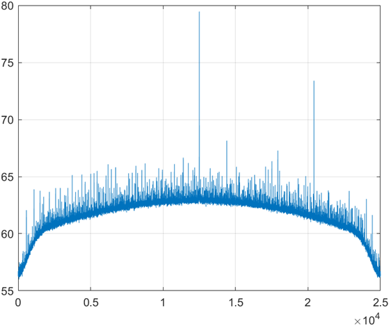
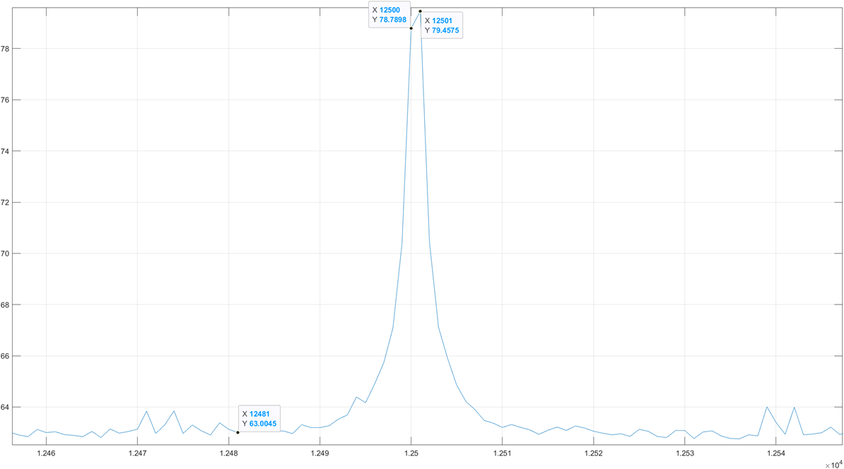
Figure 4 below show the spectrum “zoomed” at around the centre frequency (the centre of the spectrum).

The total received signal power is estimated as follows. The signal power around the spectrum peak (derived from the spectrum power in dB/kHz) is summed within ±1MHz around the peak since the signal frequency is $2MHz$ (figure 4).

Since it is a summation over several bin $/Hz$, hence the unit will be only in $dB$ instead of $dB/Hz$.

The total signal power around this ±1MHz region is about $10*log_{10}(10^{7.8} + 10^{7.9})$=$81.5 dB$ (see the points at the peak in figure 4, we convert each value into amplitude, summed them up and the scale by $10log_{10}(.)$).

Alternatively, if we want to calculate in MATLAB, we code will look like:

signal_power=sum(10.^FFT_data(index_peak-1000:index_peak+1000))
signal_power_log=log10(signal_power)

Note that at this point everything is in dB (instead of dBm since at the receiver, the signal is only process numbers).

Since we know that the generated signal power is -50dBm, then this $81.5dB$ is representing -$50dBm$ signal.

Figure 4: The total power of the received sinusoid signal and the power of the noise floor. Note that the bin size of the spectrum is 1KHz.

5. Estimate the power of the noise floor.

It is important to note that the spectrum bin width is 1kHz.

The noise floor of the spectrum is estimated by taking the median value of the spectrum (or anywhere on the “floor region” of the spectrum).

The estimated spectrum noise floor is $63dB/1KHz$.

Then, we can convert to dB/Hz as follow: $63dB/1KHz$ = $(63-30) dB/Hz$ = $33dB/Hz$.

6. estimate the C/N0 of the signal.

The C/N0 of the signal is the difference between the power of the received signal and the power of the noise floor.

The C/N0 of the signal is $81.5dB-33dB/Hz$=$48.5dB-Hz$

Hence, we can say that the received signal is $48.5dB-Hz$ above the noise floor.

7. Estimate the receiver noise.

Finally, the receiver noise is estimated as:

$the power of the generated sinusoid signal – the spectrum power above the noise floor (C/N0)$

Hence, the receiver noise is therefore = $-50dBm –48.5dB-Hz$ = $-98.5dBm/Hz$.

That is, the estimated RF receiver noise is $-98.5dBm/Hz$.

Conclusion

In this post, we have presented the basics of signal processing unit which are dB, dB-Hz and dB/Hz. Although basics, there are people who still confuse about these concepts of different units. These three types of units have fundamentally different meaning.

Then, the practical procedure to estimate the noise of RF receivers have been presented. By knowing the noise of an RF receiver, understanding of the receiver behaviour and its effect to signal processing algorithms can be estimated.

You may find some interesting items by shopping here.