Mathematical geometrical fitting: Automatic measurement algorithm case studies

In this post, practical case studies of algorithm implementations for automatic geometrical perpendicularity and cutting tool measurements are presented.

These algorithms used combination of algorithms. Some of main aspects of the automatic algorithms are fitting algorithms that have been previously discussed in this blog, that is about linear and non-linear geometrical fitting algorithms.

Data pre-processing algorithms are needed before applying fitting algorithms to solve the two case studies. One of the main pre-processing algorithms is segmentation algorithm.

Segmentation algorithm is an algorithm to select certain relevant points that will be used to calculate a measurement task at hand. This segmentation algorithm is instrumental to automate the measurement algorithm and remove operator intervention in selecting points to process.

By the end of this post, reader will learn:

• Segmentation algorithm
• Linear and non-linear fitting algorithm application
• Point cloud processing, such as point projections and curvature calculations
• Minimum-zone fitting algorithm for geometrical verification

Let us go into details!

READ MORE: Mathematical geometrical fitting: Concept and fitting methods

• Numerical Python: Scientific Computing and Data Science Applications - A book Leverage the numerical and mathematical modules in Python and its standard library

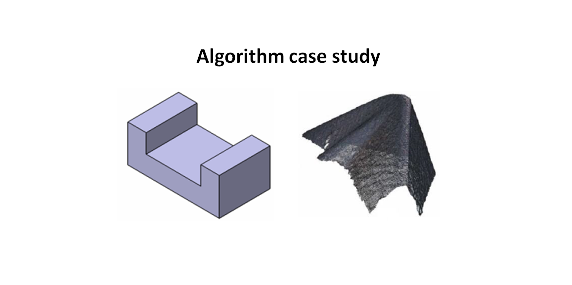
Case study 1: Algorithm for automatic measurement of perpendicularity error

Perpendicularly measurement is a type of related geometrical measurement that requires a datum. In this example, the measurement of perpendicularity of a meso-scale part with micro-scale tolerance is presented [1].

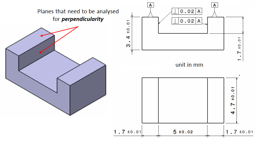
Figure 1 below shows the 3D drawing and its 2D draft with dimensions and tolerances of a part used in this case study. The perpendicularity of the two planes (shown in figure 1) will be automatically measured from measured point cloud. The perpendicularity tolerance is $0.02 mm (20 \mu m)$. The reference datum is Datum A shown in figure 1.

To get the point cloud, an optical measuring instrument is used. The instrument is focus variation microscopy (FVM).

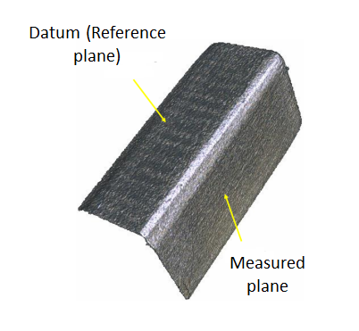
For the perpendicularity measurement, there are two planes need to be measured that are the reference plane and the plane of which the perpendicularity will be measured.

Figure 2 below shows the measured points of the required two planes. The point cloud has approximately one million points.

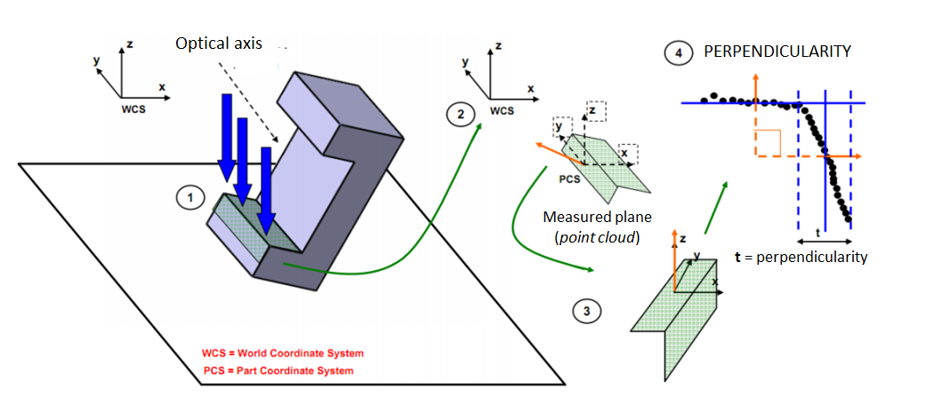
There are several steps required to automatically process the raw measured points. These steps are from data pre-processing until obtaining the perpendicularity calculation.

Figure 3 above shows the steps to automatically calculate the perpendicularity from measured points. The steps of the algorithm are as follow:

1. Perform plane fitting on the points of reference plane (figure 2) and get the unit normal vector from the reference plane $a_{ref}$.

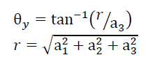
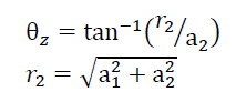
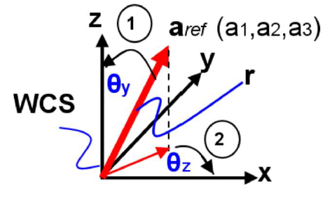
2. calculate the angle $a_{ref}$ with respect to the world coordinate system (WCS) of the measurement to get the spatial rotation angle $\theta_{y}$ and $\theta_{z}$ of the reference plane (figure 4). The calculation of the planar and spatial rotational are as follow:

3. Perform inverse rotation transform of $a_{ref}$ with respect to the spatial and planar rotation so that the part coordinate system (PCS) aligns to the WCS (step no. 3 in figure 3). The rotation is calculated as:

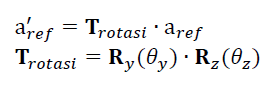
Where $\bf R _{y}(\theta _{y})$ and $\bf R _{z}(\theta _{z})$ is a rotational matrix along $y-$ and $z-$ axis.

READ MORE: Mathematical geometrical fitting: Linear geometry least-squared fitting (with tutorial)

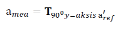
4. Perform rotation $a_{ref}’$ for 90 degree along $y$-axis. The rotation result of $a_{ref}’$ is the normal vector of the measured $a_{mea}$ (see picture 2) as follow:

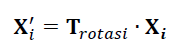
5. Perform invers transform of all the points (on the reference plane and the measured plane) with respect to the previously determined spatial rotation $\theta _{y}$ and $\theta _{z}$ as follow:

6. Perform a plane fitting on the points of the measured plane (figure 2). The point on the measured plane is the centroid (calculated as the average) of the fitted plane of the measured plane and the normal vector is $a_{mea}$.

7. Calculate the maximum distance of a point on the right and left of the fitted measured plane. The maximum distance is the perpendicularity measurement of the measured plane with respect to the reference plane.

READ MORE: Mathematical geometrical fitting: Non-linear geometry least-squared fitting (with tutorial)

• Numerical Python: Scientific Computing and Data Science Applications - A book Leverage the numerical and mathematical modules in Python and its standard library

Case study 2: Algorithm for automatic measurement of the rake angle of a cutting tool

In this section, an automatic measurement algorithm for the rake angle of a cutting tool is presented [1].

The rake angle measurement is performed by using a FVM optical CMM instrument (as in the case 1). The total measured points obtained by the instrument is 450000 points.

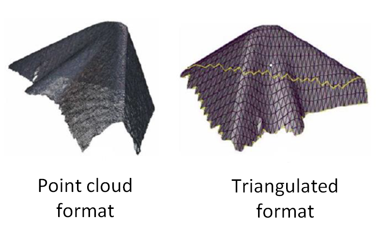
Figure 5 below shows the measurement results in spatial coordinate $X, Y$ and $Z$ format and triangulated format.

Because the measurement is performed automatically without the manual intervention of an operator, hence the measurement steps become longer than the case study 1.

One obvious reason is that, segmentation algorithm is instrumental and required to select which points that are relevant to process and to calculate the rake angle.

In this case study, the algorithm works on the triangulated format instead of the raw spatial $X,Y$ and $Z$ coordinate format. Hence, if the measurement data are still in raw $X,Y$ and $Z$ format, the data should be transformed into the triangulation format.

Triangulation format is a very common format to represent a 3D model of an object or surface.

The steps for the automatic rake angle measurement are as follow:

1. Estimate the normal vector and curvature for each point

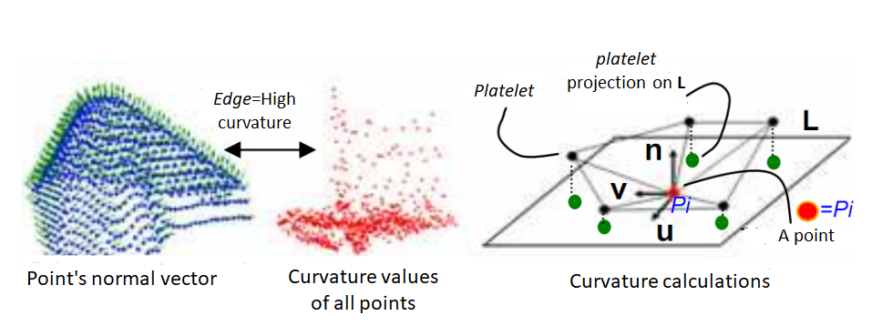
The algorithm to calculate curvature of a 3D point is based on Hamman, 1993 [2]. The steps to estimate the curvatures are illustrated in figure 6 below.

In figure 6, for each point $\bf P_{i}$, its normal vector $\bf n$ is estimated by $\sum_{i=1} ^{N} \frac{\bf n_{i}}{N}$ where $\bf n_{i}$ is the normal vector of adjacent planes at that point $\bf P_{i}$ and $N$ is the number of adjacent planes (faces) on the point $\bf P_{i}$ (Figure 6 left).

Subsequently, the average curvature $H=(k_{1}+k_{2})$ is calculated for each point $\bf P_{i}$. $k_{1}$ and $k_{2}$ are the two principle curvatures of point $\bf P_{i}$. Hence, each point on edge will have a significantly higher value of $H$ than other points that are not on the edge (figure 6 middle).

$k_{1}$ and $k_{2}$ are determined from platelets that are the adjacent points with respect to point $\bf P_{i}$ (Figure 6 right).

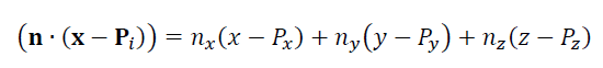
The procedure to calculate $k_{1}$ and $k_{2}$ is as follow. For each point $\bf P_{i}$, a plane $PL$ is defined in an implicit function as:

Then, $Platelet_{j}$ that are all platelets of point $\bf P_{i}$ are projected to the plane $PL$. The projection of $Platelet_{j}$ on $PL$ is called as $Platelet_{j} ^{p}$ and is calculated as:

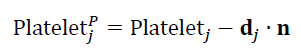
Where $\bf d_{j}$ is the orthogonal distance from $platelet_{j}$ to the plane $PL$.

All the $Platelet_{j}$ of point $\bf P_{i}$ are then translated into a new coordinate system that is centred at point $\bf P_{i}$ with a basis unit vector defined as: $<\bf u, \bf v>$.

To perform the translation, a difference vector $\bf d_{j}$ between $\bf d_{j}$ and $Platelet_{j} ^{p}$ is calculated as $\bf d_{j} =Platelet_{j} ^P-\bf d_{j}$.

This difference vector $\bf d_{j}$ can be represented in a linear combination of $<\bf u, \bf v>$ as follow:

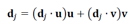
So that the local coordinate of each component $Platelet_{j} ^{p}$ based on $<\bf u, \bf v>$ is:

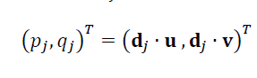
is calculated as:

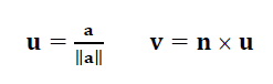
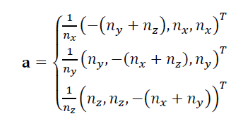
Where $\bf a$ is a vector that is perpendicular and satisfies $\bf n(a \cdot n)=0$, that is:

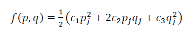
A polynomial second-degree function, $f$, that has absis and ordinate is defined as:

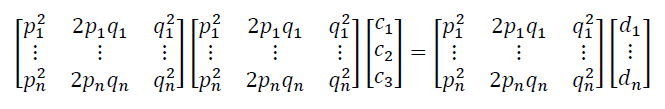
In a matrix form, the above function is represented as:

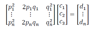
By solving the above matrix equation by using least-square method, the above equation becomes:

By solving $c_{1}, c_{2}, c_{3}$, the two principle curvatures $k_{1}$ and $ k_{2}$ can be calculated as the root of $k_{1}-(c_{1}+c_{3})k+c_{1}c_{3}-c_{2}^{2}$.

READ MORE: Mathematical geometrical fitting: Initial solution problems

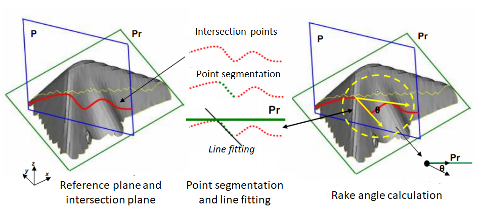
2. Construct a reference plane $\bf P_{r}$ and intersection plane $P$.

The reference plane $\bf P_{r}$ is calculated from points on edge that are identified from the curvature value of the points. To identify the edge points, points with curvature value $H>10$ are selected as points on edge.

The plane is reconstructed by determining a point on plane $\bf P_{r}$ and the vector normal of this point (figure 7 left).

To determine the plane $\bf P_{r}$, an orthogonal fitting based on least square for a plane is used. the fitting process is performed by finding the Eigen vector that corresponds to the smallest Eigen value of a matrix $\bf M$, that is a matrix containing spatial points $\bf P_{i}$ on the edge.

Where the point on plane $\bf P_{r}$ is the centroid (average) of all the points $\bf P_{i}$. The plane equation used is:

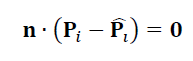
Where $ \hat{\bf P_{l}}$ is the centroid of $\bf P_{i}$.

The plane $\bf P_{r}$ (that is a plane on the edge of the cutting tool measured points) is used to calculate plane $\bf P$ (figure 7 left). This plane $\bf P$ is a plane that perpendicular to $\bf P_{r}$.

The unit vector (normal vector) of the plane $\bf P$ is calculated by rotating the unit normal vector of the plane $\bf P_{r}$ about 90 degree along the axis that is perpendicular to the edge line. The point on plane $\bf P$ is the same point on plane $\bf P_{r}$.

3. Perform point segmentation and line fitting.

The process of point segmentations is applied on intersection points between the plane $P$ and the triangulated model of the cutting tool measured points (figure 7 middle).

To get the intersection points, a parametric equation is used. A line that passes through two points $\bf Pt_{1}$ and $\bf Pt_{2}$ is defined in a parametric equation as follow:

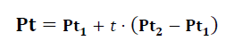
Where $t$ is a scalar quantity that is used to determine a point on the line to fit.

By inserting the above line parametric equation into the plane equation, $t$ can be calculated as:

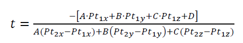
After obtaining $t$, the intersection points of the intersection plane $\bf P$ on the cutting tool measured 3D model in the triangulated format (mesh) can be calculated. Hence, the point segmentation process can be performed.

The steps of the point segmentation are as follows. Points that have a very far distance with respect to the plane $\bf P_{r}$ are neglected. Hence, the intersection points are sequenced in ascending order with respect to its $x$ and $y$ value (we can use selection sort for this sequencing process).

Then, those intersection points are checked one by one from the initial point to the last point in the sequence (figure 7 middle). The segmented points are identified as the point with the smallest $y$ coordinate value.

At least 15 points should be obtained and then form these points, a line geometry is orthogonally least square fitted. Hence, the next pint is checked, the new standard deviation of the point $\sigma _{new}$ is calculated after adding the new point. If $\sigma _{new}<\sigma _{previous}$, hence the new point is included in the set of segmented points. This process is repeated until $\sigma _{new}>\sigma _{previous}$ after adding three consecutive new points.

4. Calculate the rake angle.

Finally, the rake angle of the cutting tool can be calculated. The rake angle is the angle $\theta$ between the line, fitted from the segmented points obtained from step 3, and the intersection plane projected on plane $\bf P_{r}$ (figure 7 middle and right).

To calculate the rake angle, the unit normal vector $\bf n_{line}$ from the fitted line in step 3 is projected on plane $\bf P_{r}$ (in figure 7 right). The projection of $\bf n_{line}$ on plane $\bf P_{r}$ is calculated as:

Finally, the rake angle $\theta$ can be calculated as the angle between $\bf n_{line}$ and $\bf n_{line-projected}$.

READ MORE: Mathematical geometrical fitting: Data filtering of measurement points

• Numerical Python: Scientific Computing and Data Science Applications - A book Leverage the numerical and mathematical modules in Python and its standard library

Conclusion

The applications of measurement algorithms for automatic measurement of the perpendicularity of a part and the rake angle of a cutting tool have been presented.

The instrumental aspects of the automatic measurement algorithms are segmentation algorithm as well as line and plane fitting. Additional algorithms such as curvature estimation is also important as part of the automatic algorithms.

Form this post, we can see that algorithms have an instrumental role in dimensional and geometrical as well as surface texture measurements.

Reference

[1] Syam, W.P., 2015. Uncertainty evaluation and performance verification of a 3D geometric focus-variation measurement.

[2] Hamann, B., 1993. Curvature approximation for triangulated surfaces (pp. 139-153). Springer Vienna.

You may find some interesting items by shopping here.