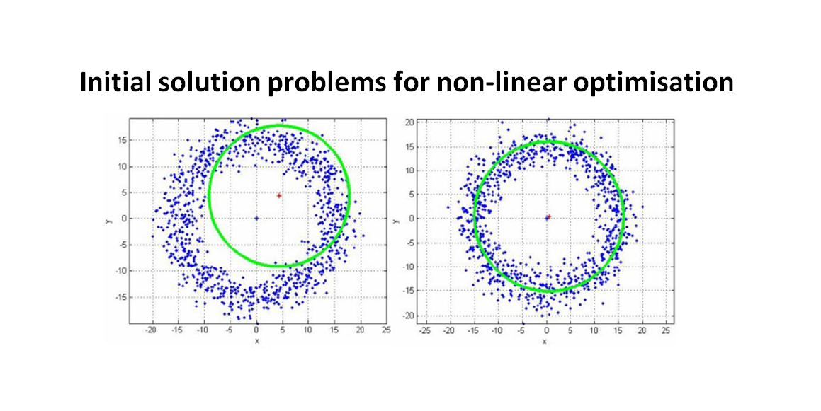
Mathematical geometrical fitting: Initial solution problems

Any iterative optimisation algorithms, used to optimise non-linear and multi-modal objective functions, always require an initial solution estimation.

The given initial solution significantly affects the final results of non-linear optimisation processes [1,2].

From these initial solutions, iterative algorithms, for example Levenberg-Marquardt algorithm, will improve the solutions on each optimisation steps until a stopping criterion is achieved.

Ideally, the given initial solutions should be as close as possible to the optimal solutions. However, in many cases this situation is impossible as very often we do not know where the optimal solutions are located within a solution search space.

READ MORE: Mathematical geometrical fitting: Concept and fitting methods

• Numerical Python: Scientific Computing and Data Science Applications - A book Leverage the numerical and mathematical modules in Python and its standard library

Initial solution estimation in Levenberg-Marquardt (LM) algorithm

As being discusses in the previous post, LM algorithm works based on linearising, by using the Taylor series expansion method, the function for searching the next candidate solution. Initially, the function to determine the next candidate solution is non-linear.

This linearisation process produces the Gauss-Newton method that is characterised by a small step to find the next candidate solutions (due to the limitation of the validity of the Taylor series expansion).

However, one of the negative effects of the linearisation is that, due to missing information on higher-order terms, the iteration steps used to find a better next candidate solution can be trapped at a local sub-optimal solution.

Being trapped in sub-optimal local optima cause the fitting of a non-linear geometry becomes non-optimal. For example, in a circle fitting, the final fitted geometry has a centre that is shifted from the original expected centre, or the diameter is smaller or bigger than the expected one.

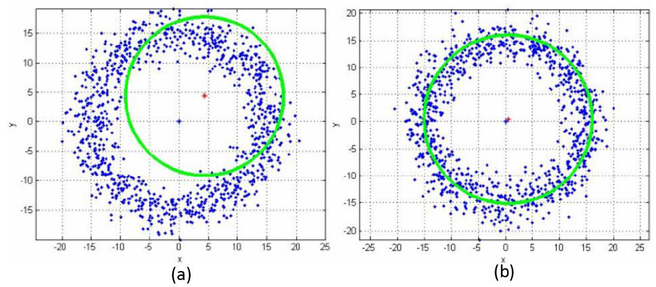
Figure 1 below show an example of circle fitting that uses different initial solutions for the parameters to fit (centre coordinate $x,y$ and its radius $r$).

In figure 1 left, the given initial solutions are far from the optimal solutions (that are the expected and known circle centre and its radius). Hence, the resulted circle fitting is not as expected. The estimated centre of the circle is shifted, and the estimated radius is smaller than expected.

In figure 1 right, the given initial solutions are close to the optimal solution. In this case, since the data is simulated, we know the nominal centre and radius of the circle (however, in many situations, these parameters are unknown!). Hence, the final estimated centre and radius of the circle are as expected and representative of the points (in blue).

From this simple example, initial solutions given for non-linear optimisation, for example for non-linear geometry fitting, are very significant for the final solutions obtained from the optimisation. The take home note is that we need to find a way to have a good estimate for initial solutions!

• Numerical Python: Scientific Computing and Data Science Applications - A book Leverage the numerical and mathematical modules in Python and its standard library

Chaos optimisation algorithm for initial solution estimation

One way to improve initial solutions for iterative algorithm of non-linear optimisations is by using chaos optimisation algorithm [2,3].

“Chaos” is mathematical defined as a semi-random property that is obtained from a non-linear equation. This non-linear equation calculates dynamical steps that are chaotic (unpredictable).

Chaos optimisation is a type of iterative-based optimisations where on each iteration step, the next solution is determined based on a chaos step (unpredictable step). By using chaotic step, there is a high probability that the optimisation step can escape from a local optima solution “trap” [4,5].

With this chaos optimisation, we can improve our initial solutions so that these initial solutions can be closer to an optimal solution than the one before improvement. Chaos optimisation will not visit the same solutions (with high probability) in its iteration step.

Chaotic motion can be generated from a non-linear model using a logistic function as follows:

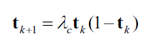
Where $\lambda \in {3.56, 4}$ is a control argument and $k$ is the iteration sequence. It is recommended that $0 \leq \bf t \leq 1$ where $\bf t_{0} \notin {0, 0.25, 0.5, 0.75, 1.0}$.

The property from the equation above is chaos in the sense of the value of $\bf t_{k}$ is unpredictable, that is, the value changed drastically in the limit of $\lambda _{c}$ and $\bf t_{k}$.

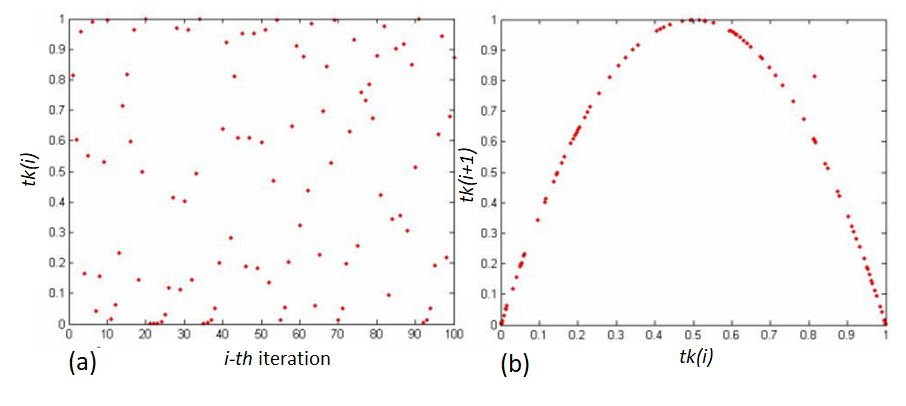
Figure 2 below shows an example of numerical chaotic motion. In figure 2 left, the plot of $\bf t_{k}$ is shown and, in figure 2 right, the pair plot between $\bf t_{k}$ and $\bf t_{k}$ is shown.

There are other non-linear functions that can generate a chaotic motion or step, for example, Tent function, Bernoulli function, Chebyshev function and others [3].

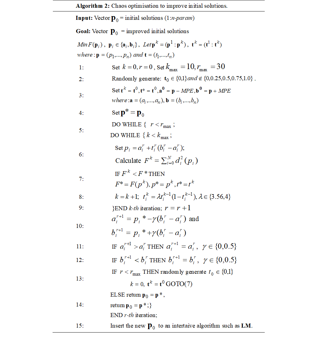
Table 1 below describes the chaos optimisation algorithm in detail for the case of non-linear geometry fitting from measured points. In table 1, the inputs for the chaos algorithm are initial solutions that are considered not yet optimised (that is, far from optimal solutions).

In table 1, MPE is maximum permissible error that described the possible error a measurement machine can have. Usually, this MPE value can be found in the specification of a measuring machine, such as tactile and optical coordinate measuring machine (CMM).

The output of the chaos optimisation algorithm is the improved version of the initial solutions that is expected to be closer to the global optimal solution. These improved initial conditions are then used as the input for an iterative optimisation algorithm, such as LM algorithm, to improve the optimisation results (in case of geometrical fitting problems, an expected or representative fitting result can be obtained).

READ MORE: Mathematical geometrical fitting: Linear geometry least-squared fitting (with tutorial)

Improvement of non-linear fitting with Chaos algorithm

Chaos optimisation algorithm can effectively improve the results of a non-linear fitting process using an iterative algorithm [2,3].

Figure 3 shows the example of an improved circle fitting by using LM algorithm combined with Chaos algorithm. In figure 3 left, we can see that the circle fitting without chaos algorithm produces a result that does not represent the measured points. The reason is that, the given initial points are far from the expected final parameter solutions.

Meanwhile, in figure 3 right, the fitting results of the circle is representative of the measured points. The fitted circle goes through the middle of the measured points and the circle centre is close to the nominal centre. In figure 3 right, the initial solutions are improved by the chaos algorithm. Hence, the LM uses these improved initial solutions and can give much better fitting solutions compared to the figure 3 left.

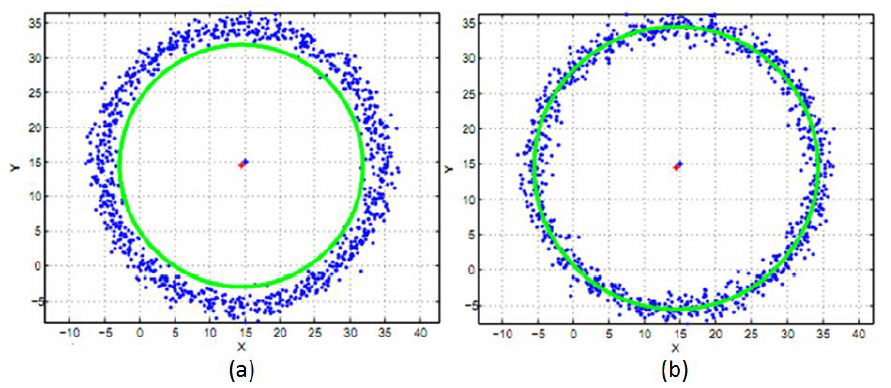
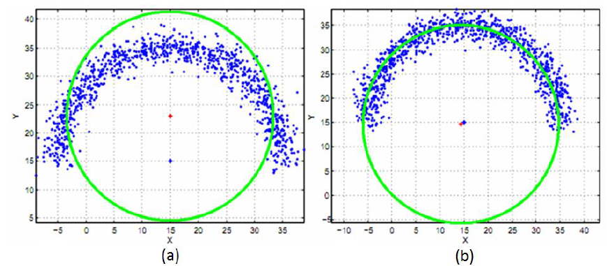
Figure 4 shows a more difficult circle fitting because the measured points only represent half of the circle. In this fitting situation, the benefit of using Chaos optimisation algorithm becomes more significant than the previous circle fitting case.

In figure 4 left, the circle fitting result by using only LM algorithm is far from nominal circle parameters. Since the measured points to fit a circle is not representing the whole circle, navigating to find the best circle parameters in the search space of the non-objective optimisation becomes difficult.

In figure 4 right, the initial solutions are then improved by utilising the chaos algorithm before being inserted into the LM algorithm. We can see that, the chaos algorithm can significantly improve the initial solutions and hence, the final circle fitting results become representative with respect to the nominal circle.

In addition, Chaos algorithm does not only improve the quality of initial solutions so that non-linear optimisation results can be improved, but also this algorithm significantly improve the computational efficiency of an iterative optimisation algorithm, such as LM algorithm.

The reason is that, when initial solutions are placed close to optimal solutions, an iterative optimisation algorithm can converge to good or optimal solutions faster because the number of iteration steps are also reduced. In addition, chaos algorithm can help avoid initial solutions being trapped or close to local optima solutions.

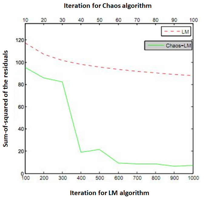
Figure 5 below shows the comparison of computational efficiency of circle fitting between LM algorithm only and LM algorithm combined with Chaos algorithm. In figure 5, we can see that the fitting process that only uses LM algorithm is trapped in a local optimum so that even though the iteration steps continue, the fitting results are not improved.

Different with the LM algorithm combined with the Chaos algorithm, this LM algorithm can escape from the local optima and can rapidly converge into good solutions.

READ MORE: Mathematical geometrical fitting: Non-linear geometry least-squared fitting (with tutorial)

Conclusion

In this post, the problem of initial solution determination for iterative algorithm is presented. Iterative algorithm is used for optimising non-linear objective function.

Bad initial solutions can significantly degrade the final solution of a non-linear optimisation. Otherwise, good initial solutions (that are close to a final global optimal solutions) can significantly improve the non-linear optimisation results as well as can reduce the computational cost of the optimisation.

Chaos algorithm used to improve initial solutions has been presented and discussed. Examples have been given to show the advantage of chaos algorithm combined with iterative LM algorithm for non-liner geometry fitting.

Chaos algorithm can improve the initial solutions for iterative LM algorithm such that the initial solutions are close to global optimal solutions and are not trapped in a local optima area in the non-linear search space.

Reference

[1] Rardin R L 2006 Optimization in Operation Research (New York: Addison-Wesley).

[2] Moroni, G., Syam, W.P. and Petrò, S., 2014. Performance improvement for optimization of the non-linear geometric fitting problem in manufacturing metrology. Measurement Science and Technology, 25(8), p.085008.

[3] Moroni, G., Syam, W.P. and Petrò, S., 2016. Comparison of chaos optimization functions for performance improvement of fitting of non-linear geometries. Measurement, 86, pp.79-92.

[4] Luo, Y.Z., Tang, G.J. and Zhou, L.N., 2008. Hybrid approach for solving systems of nonlinear equations using chaos optimization and quasi-Newton method. Applied Soft Computing, 8(2), pp.1068-1073.

[5] Tavazoei, M.S. and Haeri, M., 2007. An optimization algorithm based on chaotic behaviour and fractal nature. Journal of Computational and Applied Mathematics, 206(2), pp.1070-1081.

You may find some interesting items by shopping here.