Mathematical geometrical fitting: Non-linear geometry least-squared fitting (with tutorial)
The fitting process for non-linear geometry is more complex than that for the linear geometry fitting. Non-linear geometry includes circle (2D and 3D), sphere, cylinder, cone and torus as well as more complex geometries such as free-form surfaces.
The fitting process for non-linear geometry is more complex than that for the linear geometry fitting. Non-linear geometry includes circle (2D and 3D), sphere, cylinder, cone and torus as well as more complex geometries such as free-form surfaces.
The main reason for the complexity of non-linear geometry fitting is that the objective function of residuals of non-linear geometry cannot be linearised.
Hence, to minimise the objective function of non-linear geometry to associate nominal geometry to them, an iterative optimisation process should be performed.
The main drawbacks of this iterative method are high computational resource requirement and no guarantee to achieve global minimum solutions (as the objective function has a complex search space with many local minima).
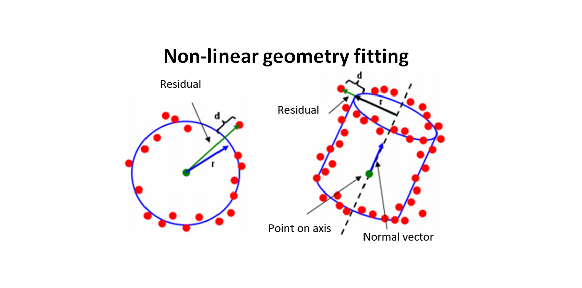
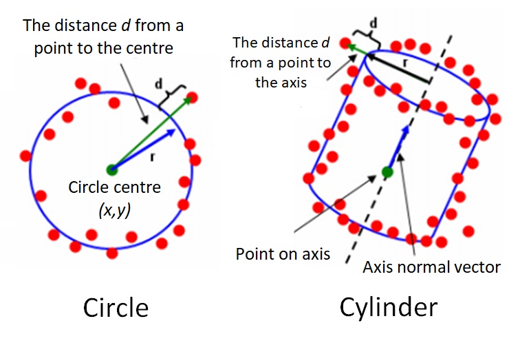
Figure 1 below shows the illustration of the residuals of a circle (representing 2D geometry) and cylinder (representing 3D geometry). In figure1, the residual is the orthogonal distance between a point to a nominal geometry.
READ MORE: Mathematical geometrical fitting: Concept and fitting methods
Least-squared fitting of circle
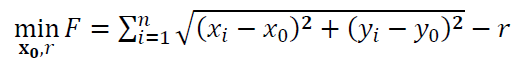
The residuals for circle fitting is (figure 1 left):

Where $\bf X_{0}$ = $[x_{0},y_{0}]^{T}$ is the circle centre to estimate or fit, $r$ is the radius of the circle to estimate or fit, $\bf X_{i}$ = $[x_{i},y_{i}]^{T}$ is the $i-th$ measured point and $||\bf X||$ is the $L_{2}$-norm of the vector $\bf X$, for example $||\bf V||$=$\sqrt{v_{1} ^{2}+ v_{2} ^{2}+ v_{3} ^{2}}$.
Hence, the objective function of the circle fitting process is:
Least-squared fitting of sphere
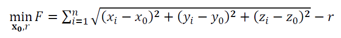
The residuals for sphere fitting is:

Where $\bf X_{0}$ = $[x_{0},y_{0}, z_{0}]^{T}$ is the sphere centre to estimate or fit, $r$ is the radius of the sphere to estimate or fit, $\bf X_{i}$ = $[x_{i},y_{i}, z_{i}]^{T}$ is the $i-th$ measured point.
Hence, the objective function of the sphere fitting process is:
Least-squared fitting of cylinder
The residuals for cylinder fitting is (figure 1 right):
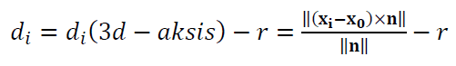
Where $d_{i}(3d-aksis)$ is the distance from a 3D point $\bf X_{i}$ to the axis (line) of a cylinder to estimate or fit and $r$ is the radius of the cylinder.
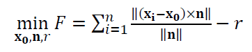
Hence, the objective function of the cylinder fitting process is:
READ MORE: Mathematical geometrical fitting: Linear geometry least-squared fitting (with tutorial)
Numerical solution for least-squared fitting of non-linear geometries
Because the objective function for the fitting of non-linear geometries cannot be linearised, an iterative optimisation algorithm should be used to perform the fitting process.
An iterative algorithm requires initial solution to start with. This initial solution can be determined by a random solution or a good estimation process for solution initialisations.
One factor that causes the non-linear fitting is more complex than linear fitting is that the non-linear fitting objective function has many minimum (optimal) solutions, that is local optima.
Non-linear optimisation processes can stop at one sub-optimal solution (local optima) and cause the fitting results is not the best solution.
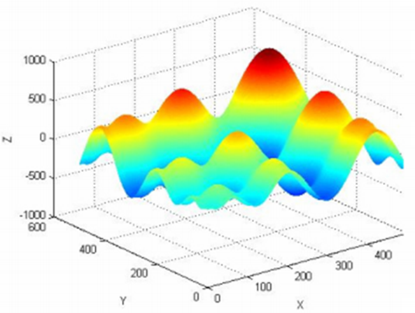
Figure 2 below shows an example of a non-linear objective function that has many local optima, that is it has many minimum and/or maximum values.
A “not good” optimisation algorithm can be trapped at one of the local optima and give sub-optimal fitting results. That is, the fitted geometry does not really fit the measured points.
Local optima condition is a situation where an iterative optimisation reach a sub-optimal solution from which the next step of the iteration process does not produce a better solution than the current solution. Hence, the optimisation will take the local optima as a final solution that is sub-optimal and stop the iteration process (the process to find the optimal solution).
A sub-optimal fitting process due to being trapped in a local optima condition will under-estimate or over-estimate the fitting process. for example, the estimated diameter of a circle is smaller than expected.
The well-known iterative algorithm to solve non-linear optimisation, and hence suitable for fitting non-linear geometries, is the Lavenberg-Marquardt (LM) algorithm.
The LM algorithm was firstly presented by Marquardt in 1963 [3]. The basic idea of LM algorithm is the combination of steepest-decent method (gradient search) and Gauss-Newton method.
The LM algorithm will work based on the steepest-decent method when the current solution is still far from an optimal solution location. Meanwhile, the LM algorithm will become Gauss-Newton method when the current solution is close to the optimal solution location.
The basic of the steepest-descent method is to find solutions based on the gradient direction of the objective function. The explanation of the steepest-decent method is as follows.
Let $F$ is the objective function to be optimised and $x_{k}$ is the current solution in the $k-th$ iteration. Hence, for the minimisation case, the next solution search is calculated as:
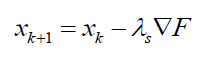
Where $ \nabla F=( \partial F/ \partial x, \partial F/ \partial y, \partial F/ \partial z)$ is the gradient of the objective function in hand and also the direction of the solution search in each iteration step. $\lambda _{s}$ is the size of the step describing how far the new candidate solution from the current candidate solution in each iteration step.
The choice for the value of $\lambda _{s}$ significantly affects the optimisation process.
Because, if $\lambda _{s}$ is set too large, hence there will be a high probability that the solution search process will jump over the optimal solution. Otherwise, if $\lambda _{s}$ is set too small, hence the solution search process will become too long to converge to an optimal solution or will never reach the optimal solution due to early stopping criteria.
The basic of the Gauss-Newton method is that the gradient of the objective function is linearised by using Taylor series expansion method.
For a non-linear objective function $F$, the Taylor series expansion for the gradient is as follows:
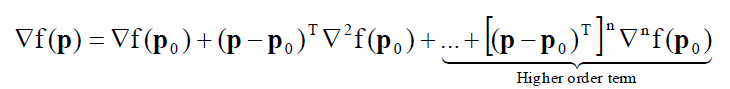
Where the “higher order term”, that is the component with exponent $>1$, is not considered, so that the Taylor series expansion equation above becomes a linear equation (being linearised).
With the linearisation of the Taylor series expansion equation above, the Gauss-Newton method/algorithm will become faster to reach a convergent solution and the mathematical function of the gradient will be easier to calculate (tractable) to find an optimal solution $\bf p$.
Vector $\bf p$ is the parameters of a non-linear geometry to be estimated.
The process to determine the next candidate solution in Gauss-Newton algorithm is by setting $\nabla F(\bf p)=0$. Hence, the next candidate solution is calculated as:
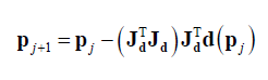
Where $\bf d(\bf p_{j})$ is the residuals at the $j-th$ iteration and $\bf J_{d}$ is the Jacobian matrix of $\bf d(\bf p_{j})$.
One important note is that the Taylor series expansion is only accurate to a small value range around the linearised point. This range is where value of the linearised function is still valid.
It means that Gauss-Newton algorithm is only effective to search an optimal solution within a very small search area within a large search space. Hence, Gauss-Newton method is only effective if initialised first solutions are already close to the optimal solutions.
The LM algorithm combines all the advantages of steepest-descent and Gauss-Newton algorithms.
The principle of Lavenberg-Marquardt (LM) algorithm
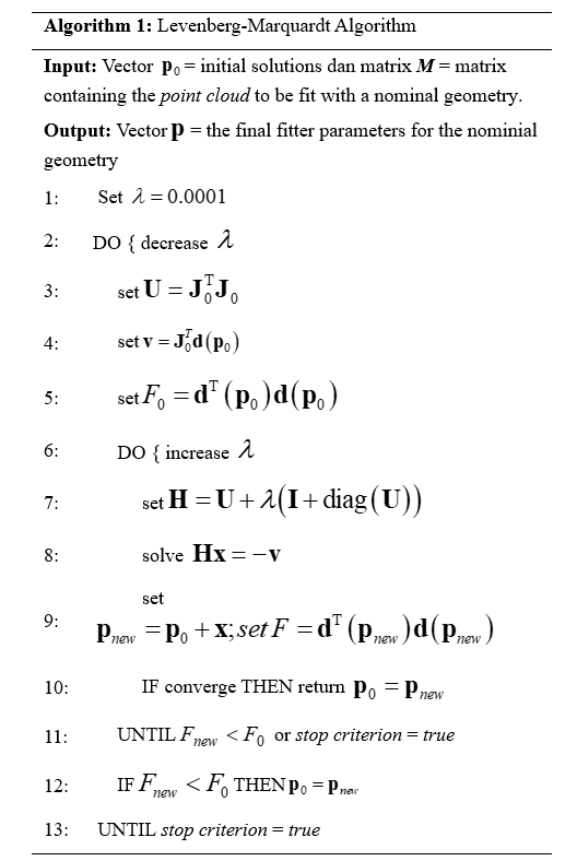
The implementation of LM algorithm proposed by Shakarji as NIST [1] is presented in Table 1 below.
In table 1, an initial solution vector $\bf p_{0}$ is generated to start the LM algorithm. A matrix $\bf M$ of $n \times 3$ size, containing the spatial coordinate of measured points to fit a nominal geometry, is the main input for the LM algorithm. Matrix $\bf M$ is defined as $[x_{1},y_{1},z_{1}; x_{2},y_{2},z_{2};…; x_{n},y_{n},z_{n}]$.
The final solution of the LM algorithm is an optimal solution vector $\bf p$ as the parameters of the fitted non-linear geometry.
The explanation of the LM algorithm is as follows (following table 1).
Let $\lambda$ is the variable in the LM algorithm and is set to decrease as much as 0.04 and to increase as much as up to 10 during the iteration steps in the LM algorithm. These values selection is based on [1].
$\bf J_{0}$ is a Jacobian matrix where the elements of the $i-th$ row is defined as $\nabla d_{i}(\bf p_{0})$.
$\nabla d_{i}(\bf p_{0})$ is the first partial derivation of $d_{i}$ with respect to each geometry parameters. The number of columns in matrix $\bf J_{0}$ is the same as the number of parameters to be estimated and the number of the row in matrix $\bf J_{0}$ is the same as the number of measured points $n$ involved in the fitting process.
The main idea of the LM algorithm lies in the equation:
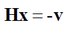
The complete form of the equation above is:
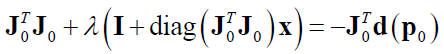
From the above complete mathematical equation (that is positive semi-definite [2]), it can be observed that when $\lambda$ has a small value, hence the LM algorithm behaves as Gauss-Newton method. Meanwhile, when $\lambda$ has a large value, hence the diagonal element of matrix $\bf J_{0}^{T} \bf J_{0}$ will be small and hence the LM algorithm behaves as steepest-descent method.
TUTORIAL: Implementation of LM algorithm for non-linear geometry fitting
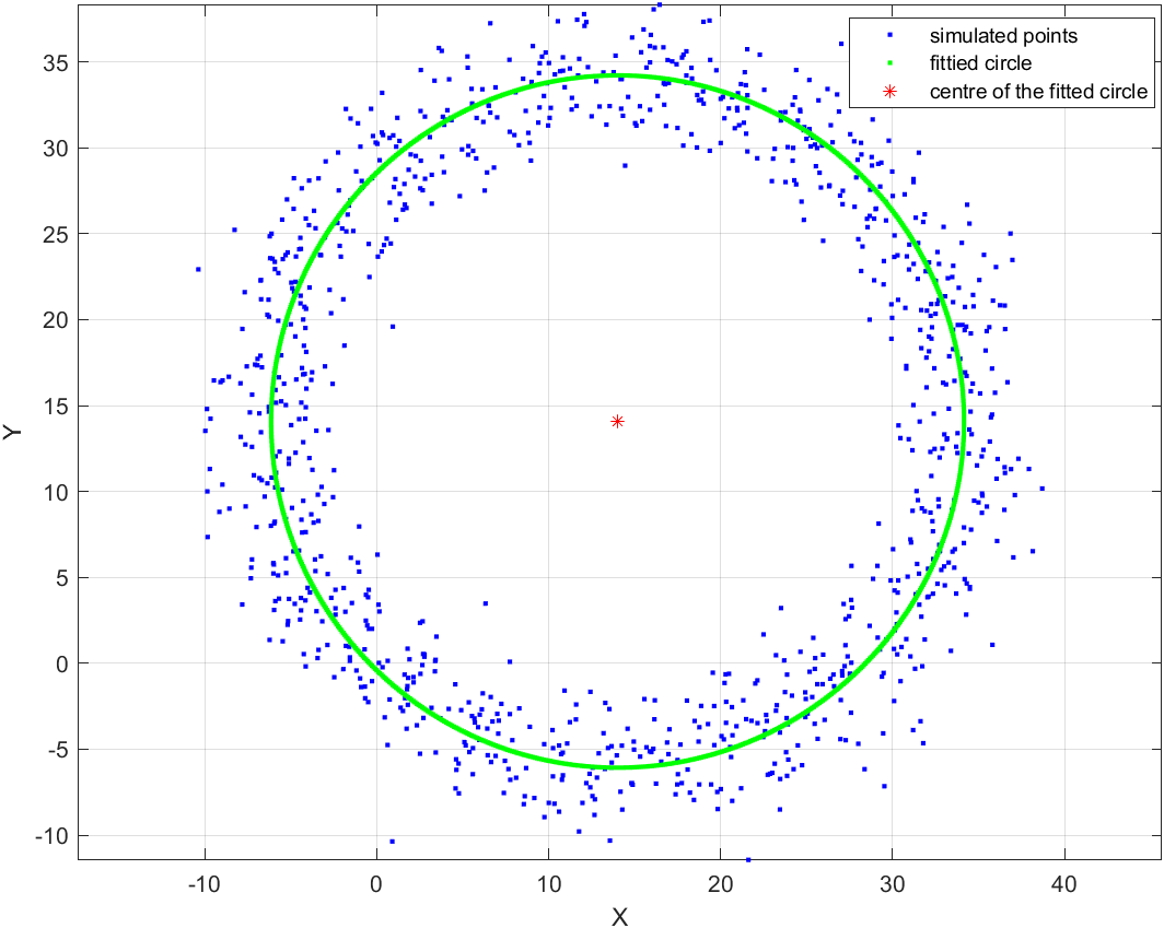
Circle fitting
The main function (point generation, function calls and plot) for circle fitting is as follows:
clc;
close all;
clear all;

%POINT GENERATION
%definition of center and radius
x1=15;
y1=15;
r= 20;

nGrid=1000;
%generate the circle
theta=linspace(0,2*pi,nGrid);
[x y]=pol2cart(theta,r);
index=1;
for i=1:nGrid
   e1=-1+2*randn;
   e2=-1+2*randn;
   x(index)=x(index)+e1;
   y(index)=y(index)+e2;
   Mraw(index,1)=x(index);
   Mraw(index,2)=y(index);
   Mraw(index,3)=1; %for homogenous coordinate
   index=index+1;
end
%translating and scaling the data
T=[1 0 x1; 0 1 y1; 0 0 1];
MrawTranslated=T*Mraw';
MrawTranslated=MrawTranslated'; %put back into original format
%----------------------------------------------------------------------

%NON-LINEAR LEAST-SQUARE CIRCLE FITTING
%for the initial point p0 of the NIST_LevMar_Spehre() function, we chose
%the center as its centroid
[n m]=size(MrawTranslated);
avgX=sum(MrawTranslated(:,1))/n;
avgY=sum(MrawTranslated(:,2))/n;
p0(1)=avgX;
p0(2)=avgY;
p0(3)=(min(MrawTranslated(:,1))+max(MrawTranslated(:,1)))/2;

points=[MrawTranslated(:,1) MrawTranslated(:,2) MrawTranslated(:,3)];
p=LevMar_Circle(p0,points) %calling the LevMar algorithm for spehre fitting
xCenterEstimated=p(1);
yCenterEstimated=p(2);
rEstimated=p(3);

%Preparing data for the fitted/estimated sphere
theta=linspace(0,2*pi,nGrid);
index=1;

R=repmat(rEstimated,nGrid,1);
[xEstimated yEstimated]=pol2cart(theta,R');
MestimatedPoints=[xEstimated' yEstimated' repmat(1,nGrid,1)];
T=[1 0  xCenterEstimated; 0 1  yCenterEstimated; 0 0 1];
MestimatedPoints=T*MestimatedPoints';
MestimatedPoints=MestimatedPoints';

%PLOTTING
%1. Generated Points
figure(1);
plot(MrawTranslated(:,1),MrawTranslated(:,2),'b.');
grid on; hold on; axis equal;

%2. Fitted Points of the circle
plot(MestimatedPoints(:,1),MestimatedPoints(:,2),'g.');
grid on; hold on;axis equal;
plot(xCenterEstimated,yCenterEstimated,'r*');
hold on;
xlabel('X');
ylabel('Y');
legend('simulated points', 'fittied circle', 'centre of the fitted circle');
axis equal;

%print error betwen the center and radius
centerError=sqrt((xCenterEstimated-x1)^2+(yCenterEstimated-y1)^2);
radiusError=abs(r-rEstimated);
fprintf('center error= %f\n',centerError);
fprintf('radius error= %f\n', radiusError);
The LM algorithm for circle fitting is as follows:
%implementation of Levenberg-Marquardt Algorithm for circle fitting
%Non-Linear Least Square
%INPUT: p0
%OUTPUT: p
%for sphere, p and p0 are center x,y,z and radius r

function p=LevMar_Circle(p0,M)
[n m]=size(M);
lamda=0.0001; %0.5;
counter1=1;
stop1=0;
while (~stop1)
    p=p0;
    lamda=lamda-0.04;

    %Build distance d vector
    for i=1:n
        d(i)=sqrt((M(i,1)-p0(1))^2+(M(i,2)-p0(2))^2)-p0(3);
    end
    %Build F0 matrix
    for i=1:n
        F0(i,1)=-(M(i,1)-p0(1))/sqrt((M(i,1)-p0(1))^2+(M(i,2)-p0(2))^2);
        F0(i,2)=-(M(i,2)-p0(2))/sqrt((M(i,1)-p0(1))^2+(M(i,2)-p0(2))^2);
        F0(i,3)=-1;
    end
    size(d);
    size(F0);
    %calculate matrix U mxm = F0'F0 where m=4 (x,y,z,r)
    U=F0'*F0;
    %calculate vector v mx1=F0'*d where m=4 (x,y,z,r)
    v=F0'*d';
    %calculate J0=sum (d^2)
    j0=sum(d.^2);

    stop2=0;
    counter2=1;
    while (~stop2)
        lamda=lamda+1;
        [n1 m1]=size(U);
        H=U+lamda*(eye(m1)+diag(diag(U)));
        %solving Hx=-v by using Cholesky decomposition
        R=chol(H);
        x=inv(R'*R)*-v;
        pnew=p0'+x;
        for i=1:n
            d(i)=sqrt((M(i,1)-pnew(1))^2+(M(i,2)-pnew(2))^2)-pnew(3);
        end
        Jnew=sum(d.^2);
        if((pnew(1)==p0(1)) &&(pnew(2)==p0(2))&&(pnew(3)==p0(3)) ) %if converge Pnew=P0 --> stop
            p0=pnew;
            p=p0;
            return;
        end

        if(Jnew<j0)
            stop2=1;
        end
        counter2=counter2+1;
        if(counter2>10000)
            stop2=1;
        end
    end %END OF INNER WHILE LOOP

    if(Jnew<j0)
        p0=pnew';  %p0 original format is a row vector
    end
    counter1=counter1+1;
    if(counter1>5000)
        stop1=1;
    end
end %END OF OUTER WHILE LOOP

%p=p0;
end %END OF FUNCTION
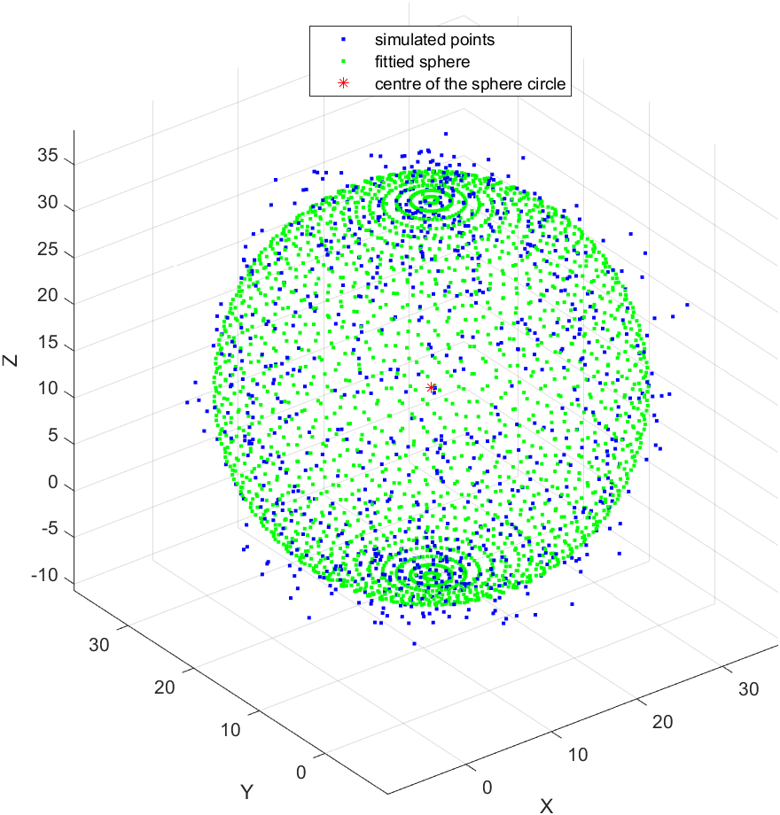
Sphere fitting
The main function (point generation, function calls and plot) for circle sphere is as follows:
clc;
close all;
clear all;


%POINT GENERATION
%definition of center and radius
x1=15;
y1=15;
z1=15;
r= 20;

nGrid=30;
%generate the sphere
[x,y,z]=sphere(nGrid);
index=1;
for i=1:nGrid+1
    for j=1:nGrid+1
        e1=-0.05+0.1*randn;
        e2=-0.05+0.1*randn;
        e3=-0.05+0.1*randn;
        x(index)=x(index)+e1;
        y(index)=y(index)+e2;
        z(index)=  z(index)+e3;
        Mraw(index,1)=x(index);
        Mraw(index,2)=y(index);
        Mraw(index,3)=z(index);
        Mraw(index,4)=1; %for homogenous coordinate
        index=index+1;
    end
end
%translating and scaling the data
T=[r 0 0 x1; 0 r 0 y1; 0 0 r z1; 0 0 0 1];
MrawTranslated=T*Mraw';
MrawTranslated=MrawTranslated'; %put back into original format
%----------------------------------------------------------------------

%NON-LINEAR LEAST-SQUARE SPHERE FITTING
%for the initial point p0 of the NIST_LevMar_Spehre() function, we chose
%the center as its centroid
[n m]=size(MrawTranslated);
avgX=sum(MrawTranslated(:,1))/n;
avgY=sum(MrawTranslated(:,2))/n;
avgZ=sum(MrawTranslated(:,3))/n;
p0(1)=avgX;
p0(2)=avgY;
p0(3)=avgZ;
p0(4)=(min(MrawTranslated(:,3))+max(MrawTranslated(:,3)))/2;
p0

points=[MrawTranslated(:,1) MrawTranslated(:,2) MrawTranslated(:,3)];
p=LevMar_Sphere(p0,points) %calling the LevMar algorithm for spehre fitting

xCenterEstimated=p(1);
yCenterEstimated=p(2);
zCenterEstimated=p(3);
rEstimated=p(4);

%Preparing data for the fitted/estimated sphere
phi=linspace(0,2*pi,50);
theta=linspace(0,2*pi,50);
[PHI THETA]=meshgrid(phi,theta);
clear phi;
clear theta;
index=1;
for i=1:50
    for j=1:50
        phi(index)=PHI(i,j);
        theta(index)=THETA(i,j);
        index=index+1;
    end
end

R=repmat(rEstimated,2500,1);
[xEstimated yEstimated zEstimated]=sph2cart(phi,theta,R');
MestimatedPoints=[xEstimated' yEstimated' zEstimated' repmat(1,2500,1)];

T=[1 0 0 xCenterEstimated; 0 1 0 yCenterEstimated; 0 0 1 zCenterEstimated; 0 0 0 1];
MestimatedPoints=T*MestimatedPoints';
MestimatedPoints=MestimatedPoints';

%PLOTTING
%1. Generated Points
figure(1);
plot3(MrawTranslated(:,1),MrawTranslated(:,2),MrawTranslated(:,3),'b.');
grid on; hold on;

%2. Fitted Points of the sphere
%figure;
hold on;
%plot3(xEstimated',yEstimated',zEstimated','b.');
plot3(MestimatedPoints(:,1),MestimatedPoints(:,2),MestimatedPoints(:,3),'g.');
grid on; hold on;axis equal;
plot3(xCenterEstimated,yCenterEstimated,zCenterEstimated,'r*');
xlabel('X');
ylabel('Y');
zlabel('Z');
legend('simulated points', 'fittied sphere', 'centre of the sphere circle');
axis equal;

%print error betwen the center and radius
centerError=sqrt((xCenterEstimated-x1)^2+(yCenterEstimated-y1)^2+(zCenterEstimated-z1)^2);
radiusError=abs(r-rEstimated);
fprintf('center error= %f\n',centerError);
fprintf('radius error= %f\n', radiusError);
The LM algorithm for sphere fitting is as follows:
%implementation of NIST Levenberg-Marquardt Algorithm for fitting
%Non-Linear Least Square
%INPUT: p0
%OUTPUT: p
%for sphere, p and p0 are center x,y,z and radius r

function p=LevMar_Sphere(p0,M)
[n m]=size(M);
lamda=0.0001;
counter1=1;
stop1=0;
while (~stop1)
    p=p0;
    lamda=lamda-0.04;

    %Build distance d vector
    for i=1:n
        d(i)=sqrt((M(i,1)-p0(1))^2+(M(i,2)-p0(2))^2+(M(i,3)-p0(3))^2)-p0(4);
    end
    %Build F0 matrix
    for i=1:n
        F0(i,1)=-(M(i,1)-p0(1))/sqrt((M(i,1)-p0(1))^2+(M(i,2)-p0(2))^2+(M(i,3)-p0(3))^2);
        F0(i,2)=-(M(i,2)-p0(2))/sqrt((M(i,1)-p0(1))^2+(M(i,2)-p0(2))^2+(M(i,3)-p0(3))^2);
        F0(i,3)=-(M(i,3)-p0(3))/sqrt((M(i,1)-p0(1))^2+(M(i,2)-p0(2))^2+(M(i,3)-p0(3))^2);
        F0(i,4)=-1;
    end
    size(d);
    size(F0);
    %calculate matrix U mxm = F0'F0 where m=4 (x,y,z,r)
    U=F0'*F0;
    %calculate vector v mx1=F0'*d where m=4 (x,y,z,r)
    v=F0'*d';
    %calculate J0=sum (d^2)
    j0=sum(d.^2);

    stop2=0;
    counter2=1;
    while (~stop2)
        lamda=lamda+1;
        [n1 m1]=size(U);
        H=U+lamda*(eye(m1)+diag(diag(U)));
        %solving Hx=-v by using Cholesky decomposition
        R=chol(H);
        x=inv(R'*R)*-v;
        pnew=p0'+x;
        for i=1:n
            d(i)=sqrt((M(i,1)-pnew(1))^2+(M(i,2)-pnew(2))^2+(M(i,3)-pnew(3))^2)-pnew(4);
        end
        Jnew=sum(d.^2);
        if((pnew(1)==p0(1)) &&(pnew(2)==p0(2))&&(pnew(3)==p0(3))&&(pnew(4)==p0(4)) ) %if converge Pnew=P0 --> stop
            %p0 from normalized pnew
            p0=pnew;
            p=p0;
            return;
        end

        if(Jnew<j0)
            stop2=1;
        end
        counter2=counter2+1;
        if(counter2>10000)
            stop2=1;
        end
    end %END OF INNER WHILE LOOP

    if(Jnew<j0)
        p0=pnew';  %put p0 original format back to a "row vector"
    end
    counter1=counter1+1;
    if(counter1>1000)
        stop1=1;
    end
end %END OF OUTER WHILE LOOP

%p=p0;
end %END OF FUNCTION
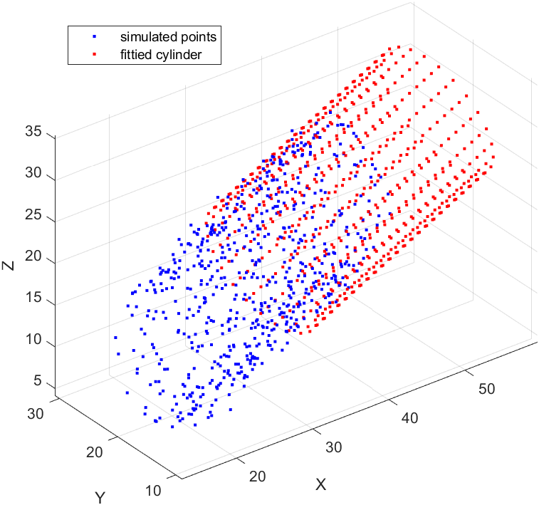
Cylinder fitting
The main function (point generation, function calls and plot) for cylinder fitting is as follows:
clc;
close all;
clear all;


%POINT GENERATION
%definition of initial parameter for cylinder
%NOTE: x,y,z for the translation, A for the rotation
x1=15;
y1=15;
z1=15;
A1=[2 4 10]; %the cylinder direction is 1i+1j+1z
r=10;
A_init=A1;

nGrid=25;
%generate the Cylinder
theta=linspace(0,2*pi,nGrid);
index=1;
for i=1:nGrid
    [x,y,z]=pol2cart(theta',repmat(r,nGrid,1),repmat(i,nGrid,1));
    for j=1:nGrid
        e1=-0.5+1*randn;
        e2=-0.5+1*randn;
        e3=-0.5+1*randn;
        x(j)=x(j)+e1;
        y(j)=y(j)+e2;
        z(j)= z(j)+e3;
        Mraw(index,1)=x(j);
        Mraw(index,2)=y(j);
        Mraw(index,3)=z(j);
        Mraw(index,4)=1; %for homogenous coordinate
        index=index+1;
    end
end
%translating and rotating the data
%NOTE: first Translate and then rotate
Rtz=[cos(atan(A1(2)/A1(1))) -sin(atan(A1(2)/A1(1))) 0 0; sin(atan(A1(2)/A1(1))) cos(atan(A1(2)/A1(1))) 0 0; 0 0 1 0; 0 0 0 1]
Rty=[cos(atan(A1(3)/A1(1))) 0 sin(atan(A1(3)/A1(1))) 0; 0 1 0 0; -sin(atan(A1(3)/A1(1))) 0 cos(atan(A1(3)/A1(1))) 0; 0 0 0 1];
Rtx=[1 0 0 0; 0 cos(atan(A1(3)/A1(2))) -sin(atan(A1(3)/A1(2))) 0; 0 cos(atan(A1(3)/A1(2))) sin(atan(A1(3)/A1(2))) 0; 0 0 0 1];
Tr=[1 0 0 x1; 0 1 0 y1; 0 0 1 z1; 0 0 0 1];
T=Tr*Rtz*Rty*Rtx;
MrawTransformed=T*Mraw';
MrawTransformed=MrawTransformed'; %put back into original format


%NON-LINEAR LEAST-SQUARE SPHERE FITTING - NIST ALGORITHM
%for the initial point p0 of the NIST_LevMar_Spehre() function, we chose
%the center as its centroid
[n m]=size(MrawTransformed);
avgX=sum(MrawTransformed(:,1))/n;
avgY=sum(MrawTransformed(:,2))/n;
avgZ=sum(MrawTransformed(:,3))/n;
p0(1)=avgX;
p0(2)=avgY;
p0(3)=avgZ;
p0(4)=2;
p0(5)=2;
p0(6)=6;
p0(7)=5;

p0
points=[MrawTransformed(:,1) MrawTransformed(:,2) MrawTransformed(:,3)];
p=LevMar_Cylinder(p0,points) %calling the LevMar algorithm for spehre fitting

xEstimated=p(1);
yEstimated=p(2);
zEstimated=p(3);
A1(1)=p(4); %value of vector A1 after LSQ estimation process
A1(2)=p(5);
A1(3)=p(6);
rEstimated=p(7);
A_opt=A1;

%Preparing data for the fitted/estimated Cylinder
nGrid=25;
theta=linspace(0,2*pi,nGrid);
index=1;
for i=1:nGrid
    [x,y,z]=pol2cart(theta',repmat(rEstimated,nGrid,1),repmat(i,nGrid,1));
    for j=1:nGrid
        M_est(index,1)=x(j);
        M_est(index,2)=y(j);
        M_est(index,3)=z(j);
        M_est(index,4)=1; %for homogenous coordinate
        index=index+1;
    end
end
%translating and rotating the data
%NOTE: first Translate and then rotate
Rtz=[cos(atan(A1(2)/A1(1))) -sin(atan(A1(2)/A1(1))) 0 0; sin(atan(A1(2)/A1(1))) cos(atan(A1(2)/A1(1))) 0 0; 0 0 1 0; 0 0 0 1]
Rty=[cos(atan(A1(3)/A1(1))) 0 sin(atan(A1(3)/A1(1))) 0; 0 1 0 0; -sin(atan(A1(3)/A1(1))) 0 cos(atan(A1(3)/A1(1))) 0; 0 0 0 1];
Rtx=[1 0 0 0; 0 cos(atan(A1(3)/A1(2))) -sin(atan(A1(3)/A1(2))) 0; 0 cos(atan(A1(3)/A1(2))) sin(atan(A1(3)/A1(2))) 0; 0 0 0 1];
Tr=[1 0 0 xEstimated; 0 1 0 yEstimated; 0 0 1 zEstimated; 0 0 0 1];
%Tr=[1 0 0 x1; 0 1 0 y1; 0 0 1 z1; 0 0 0 1]; %Just for vosualize the cylinder such that the estimated cylinder has the same origin
T=Tr*Rtz*Rty*Rtx;
M_estTransformed=T*M_est';
M_estTransformed=M_estTransformed'; %put back into original format

%PLOTTING
%1. Generated Points
figure(1);
plot3(MrawTransformed(:,1),MrawTransformed(:,2),MrawTransformed(:,3),'b.');
grid on; hold on;

%2. Fitted Points of the Cylinder
%figure;
hold on;
%plot3(xEstimated',yEstimated',zEstimated','b.');
plot3(M_estTransformed(:,1),M_estTransformed(:,2),M_estTransformed(:,3),'r.');
grid on; hold on;axis equal;
xlabel('X');
ylabel('Y');
zlabel('Z');
legend('simulated points', 'fittied cylinder');
axis equal;

%print error betwen the origin and radius
originError=sqrt((xEstimated-x1)^2+(yEstimated-y1)^2+(zEstimated-z1)^2);
A_Error=sqrt((A_init(1)-A_opt(1))^2+(A_init(1)-A_opt(1))^2+(A_init(1)-A_opt(1))^2);
radiusError=abs(r-rEstimated);
fprintf('center error= %f\n',originError);
fprintf('A error= %f\n',A_Error);
fprintf('radius error= %f\n', radiusError);
The LM algorithm for cylinder fitting is as follows:
%implementation of NIST Levenberg-Marquardt Algorithm for fitting
%Non-Linear Least Square
%INPUT: p0
%OUTPUT: p
%for sphere, p and p0 are center x,y,z and radius r

function p=LevMar_Cylinder(p0,M)
[n m]=size(M);
lamda=0.0001;
firstStep=1;
counter1=1;
stop1=0;
while (~stop1)
    p=p0;
    lamda=lamda-0.04;

    %calculate vector a=A/|A|
    lengthA=sqrt(p0(4)^2+p0(5)^2+p0(6)^2);
    a(1)=p0(4)/lengthA; %a
    a(2)=p0(5)/lengthA; %b
    a(3)=p0(6)/lengthA; %c

    %Calculate distance vector d(i) and matrix F0
    for i=1:n
        %calculate gi=a.(xi-x) --> scalar
        g(i)=a(1)*(M(i,1)-p0(1))+a(2)*(M(i,2)-p0(2))+a(3)*(M(i,3)-p0(3));

        %calculate fi=sqrt(u^2+v^2+w^2) --> scalar
        uSquare=(a(3)*(M(i,2)-p0(2))-a(2)*(M(i,3)-p0(3)))^2;
        vSquare=(a(1)*(M(i,3)-p0(3))-a(3)*(M(i,1)-p0(1)))^2;
        wSquare=(a(2)*(M(i,1)-p0(1))-a(1)*(M(i,2)-p0(2)))^2;
        f(i)=sqrt(uSquare+vSquare+wSquare);

        %calcualte distance d
        d(i)=f(i)-p0(7);

        %calculate matrix F
        if(f(i)~=0)
            F0(i,1)=(a(1)*g(i)-(M(i,1)-p0(1)))/f(i);
            F0(i,2)=(a(2)*g(i)-(M(i,2)-p0(2)))/f(i);
            F0(i,3)=(a(3)*g(i)-(M(i,3)-p0(3)))/f(i);
            F0(i,4)=g(i)*(a(1)*g(i)-(M(i,1)-p0(1)))/f(i);;
            F0(i,5)=g(i)*(a(2)*g(i)-(M(i,2)-p0(2)))/f(i);
            F0(i,6)=g(i)*(a(3)*g(i)-(M(i,3)-p0(3)))/f(i);
        else %f(i)=0
            F0(i,1)=sqrt(1-a(1)^2);
            F0(i,2)=sqrt(1-a(2)^2);
            F0(i,3)=sqrt(1-a(3)^2);
            F0(i,4)=g(i)*sqrt(1-a(1)^2);
            F0(i,5)=g(i)*sqrt(1-a(2)^2);
            F0(i,6)=g(i)*sqrt(1-a(3)^2);
        end
        F0(i,7)=-1;
    end
    size(d);
    size(F0);
    %calculate matrix U mxm = F0'F0 where m=4 (x,y,z,r)
    U=F0'*F0;
    %calculate vector v mx1=F0'*d where m=4 (x,y,z,r)
    v=F0'*d';
    %calculate J0=sum (d^2)
    j0=sum(d.^2);

    stop2=0;
    counter2=1;
    while (~stop2)
        lamda=lamda+1;
        [n1 m1]=size(U);
        H=U+lamda*(eye(m1)+diag(diag(U)));
        %solving Hx=-v by using Cholesky decomposition
        R=chol(H);
        x=inv(R'*R)*-v;
        pnew=p0'+x;
        for i=1:n
            %calculate gi=a.(xi-x) --> scalar
            g(i)=a(1)*(M(i,1)-pnew(1))+a(2)*(M(i,2)-pnew(2))+a(3)*(M(i,3)-pnew(3));

            %calculate fi=sqrt(u^2+v^2+w^2) --> scalar
            uSquare=(a(3)*(M(i,2)-pnew(2))-a(2)*(M(i,3)-pnew(3)))^2;
            vSquare=(a(1)*(M(i,3)-pnew(3))-a(3)*(M(i,1)-pnew(1)))^2;
            wSquare=(a(2)*(M(i,1)-pnew(1))-a(1)*(M(i,2)-pnew(2)))^2;
            f(i)=sqrt(uSquare+vSquare+wSquare);

            %calcualte distance d
            d(i)=f(i)-pnew(7);
        end
        Jnew=sum(d.^2);
        if((pnew(1)==p0(1)) &&(pnew(2)==p0(2))&&(pnew(3)==p0(3))&&(pnew(4)==p0(4))&&(pnew(5)==p0(5)) &&(pnew(6)==p0(6) && (pnew(7)==p0(7))) ) %if converge Pnew=P0 --> stop
            %p0 from normalized pnew
            p0=pnew;
            p=p0;
            return;
        end

        if(Jnew<j0)
            stop2=1;
        end
        counter2=counter2+1;
        if(counter2>2000)
            stop2=1;
        end
    end %END OF INNER WHILE LOOP


    if(Jnew<j0)
        origin=[p0(1) p0(2) p0(3)]'; %column vector
        p0=pnew';  %put p0 original format back to a "row vector"
    end
    counter1=counter1+1;
    if(counter1>2000)
        stop1=1;
    end

end %END OF OUTER WHILE LOOP

%p=p0;
end %END OF FUNCTION
Conclusion
In this post, non-linear geometry fitting problems have been discussed. Non-linear geometries include circle, sphere, cylinder, cone, torus and more complex geometry or feature, such as free-form surfaces.
Since the objective function is non-linear and cannot be linearised. An iterative optimisation method should be used to solve the optimisation problem of the non-linear fitting.
The fundamental idea of non-linear geometric fitting is that their non-linear gradient of the objective function is linearised by applying Taylor series expansion. With the linearisation, a Gauss-Newton search step to find a next candidate solution can be obtained.
A well-known Lavenberg-Marquardt (LM) algorithm is used to solve the non-liner geometry fitting problems. The essence of LM algorithm is that it combines the advantages of steepest-descent and Gauss-Newton methods.
Reference
[1] Shakarji, C.M., 1998. Least-squares fitting algorithms of the NIST algorithm testing system. Journal of research of the National Institute of Standards and Technology, 103(6), p.633.
[2] Nash, J.C., 1990. Compact numerical methods for computers: linear algebra and function minimisation. CRC press.
[3] Marquardt, D.W., 1963. An algorithm for least-squares estimation of nonlinear parameters. Journal of the society for Industrial and Applied Mathematics, 11(2), pp.431-441.
You may find some interesting items by shopping here.