GNSS

The importance of GNSS satellite clock-bias and orbit correction

The position of a receiver calculated from global navigation satellite system (GNSS) signals is significantly affected by the accuracy of the satellite clock-bias and orbit transmitted by GNSS satellites.

Wahyudin Syam

Dec 8, 2023 • 10 min read

The calculated position of the receiver significantly depends on the estimated pseudorange, which is significantly affected by receiver and satellite clock-bias between satellites and the receiver, and the estimated satellite orbits in view from which the position is calculated.

For example, in term of satellite clock-bias, a $10ns$ clock-bias will transform into around $3m$ pseudorange error. However, due to complex satellite internal and external factors, this clock bias may be more than $10 ns$.

Similar to satellite clock-bias, the satellite orbits, calculated from ephemeris broadcasted in GNSS satellite navigation messages, deviate from its true position about few or more metres due to internal and external factors that affect the dynamics of satellites.

In this post, we will discuss about the importance of satellite clock-bias and orbit estimation, internal and external factors affecting satellite clock-bias and orbits, machine learning (ML) methods to estimate satellite clock-bias and orbit correction as well as some results from the ML correction estimations.

Global Positioning System: Signals, Measurements, and Performance - an excellent GPS and GNSS book for modelling

How satellite clock-bias and orbit affect position estimations

To understand how satellite clock-bias and orbit fundamentally affect the calculated position of a receiver (either dynamic or static), we can have a look at the general system of equation that relates pseudorange and satellite orbit as follow:

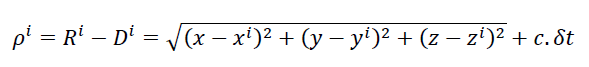
Where , $\rho $ is the estimated pseudorange of i-th satellite to the receiver, $𝑅$ is the ranging measurement between the 𝑖−𝑡ℎ satellite and receiver, $𝐷$ is ranging due to delay when the signal travels in space (for example, due to Ionospheric delay, tropospheric delay, multipath and other factors) from the 𝑖−𝑡ℎ satellite to the receiver, $\delta $ is the systematic receiver clock offset, $(𝑥,𝑦,𝑧)$ are the receiver position, $(𝑥𝑖,𝑦𝑖,𝑧𝑖)$ are the 𝑖−𝑡ℎ satellite orbit, 𝑖=1,2,⋯,𝑛 is the index of satellite and $𝑛≥4$ to solve the $x,y,z$ coordinate and clock offset $\delta $ of a receiver and $c$ is the speed of light.

To solve the above equation, a linearisation of Taylor series at around a location $(𝑥_{0},𝑦_{0},𝑧_{0})$ is applied to the non-linear code pseudorange measurement equation above to create a system of linear equations.

Since there are four unknown variables, we need at least for satellites (equations) to solve the unknown parameters. To have a least square estimate, at least five satellites (equations) should be used.

This system of linear equations is arranged in a matrix form as follow:

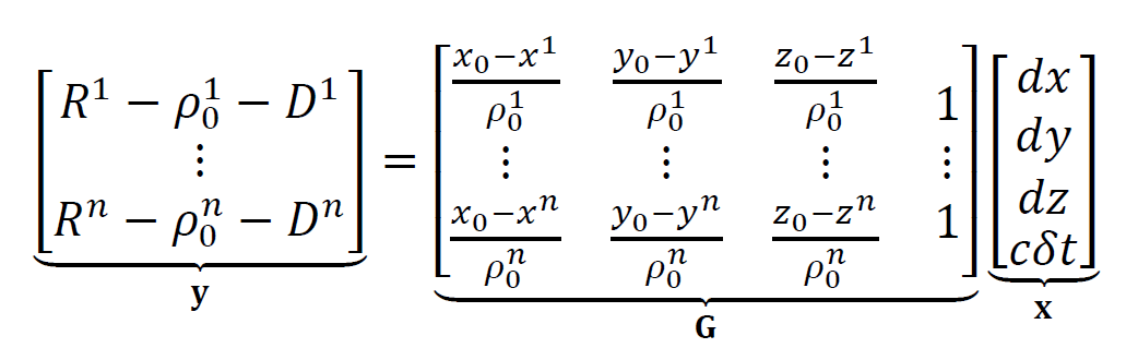
Where G is the geometry matrix, 𝐲 is the residuals between the measured and predicted pseudorange and 𝐱 is the unknown parameters to fit or solve. $(𝑥_{0},𝑦_{0},𝑧_{0})$ is the initial location that can be determined with certain rules, such as the centre location of the earth or an approximate or rough estimate of the receiver position, $\rho_{0}$.

Finally the receiver location is calculated as:

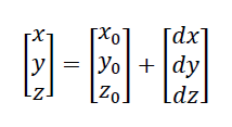
From the equations above, it is clear that the information of accurate satellite orbit is instrumental in determining the receiver position.

Regarding the pseudorange $\rho$, its estimation directly depends on the estimate of the signal travel time from a satellite that transmits the signal to a GNSS receiver.

Satellite orbit is calculated from satellite ephemeris decoded from inside the navigation message of GNSS signals.

Figure 1 below shows the schematic view of various factors affecting the signal travel time.

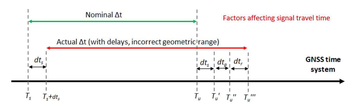
Figure 1: Timeline diagram of the total travel time of GNSS signals from an SV to a receiver in nominal (no delay and error) and actual (with delays) conditions.

In figure 1 above,$𝑇_{𝑠}$ is the time when the satellite transmits the signal at GNSS system time. $𝑑𝑇_{𝑠}$ is the clock-bias (offset) of the satellite from the GNSS system time. $𝑇_{𝑢}$ is the time when the signal arrives at a receiver without any delay. $\Delta 𝑡$ is the total signal travel time without any geometric range time error. $𝑑𝑇_{𝑝}$ and $𝑑𝑇_{𝑟}$ are signal propagation delay due to, for example, ionosphere, troposphere and multipath effects, and receiver clock-offset, respectively. 𝑇𝑢′,𝑇𝑢′′ and 𝑇𝑢′′′ are the time, with respect to the system (receiver) time, when the signal arrives at the receiver with satellite clock-bias, propagation delay and receiver clock offset, respectively.

Hence, from figure 1, the total travel time of the signal deviates from its true travel time due to the mentioned various delay.

From figure 1, the satellite clock-bias $𝑑𝑇_{𝑠}$ from the reference GNSS time system is one of the important delay sources. Hence, this clock-bias should be accurately determined to estimate the true signal transmit time $𝑇_{𝑠}$ with respect to the time system.

The satellite clock-bias is broadcasted in the navigation message of GNSS signals. This broadcasted clock-bias should be used to estimate the true signal transmit time $𝑇_{𝑠}$ as follow:

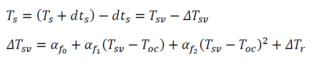
Where $𝑇_{𝑠𝑣}$ = (𝑇𝑠+𝑑𝑡𝑠) is the signal transmit time from the satellite affected by the satellite clock-bias. $\Delta 𝑇_{𝑠𝑣}$ is the estimated clock-bias broadcasted by the satellite in its navigation message, $\alpha 𝑓_{0}$, $\alpha 𝑓_{1}$ and $\alpha 𝑓_{2}$ are SV clock bias, SV clock drift and SV clock drift rate, respectively, $𝑇_{𝑜𝑐}$ is time of clock and $\Delta 𝑇_{𝑟}$ is relativistic correction time.

From the equation above, the satellite clock-bias is instrumental for the receiver position calculation and this clock-bias estimate is affected by non-linear effects such as satellite dynamics that is affected by both satellite internal and external factors.

Satellite internal and external factors affecting satellite clock-bias and orbit

The satellite orbit and clock-bias are affected by both internal and external factors.

The internal factors such as the PRN identity (related to the generation of technology state of the satellite), the satellite orbit and clock-bias estimate from master ground controls, the clock quality or clock types on-board on satellites and other factors.

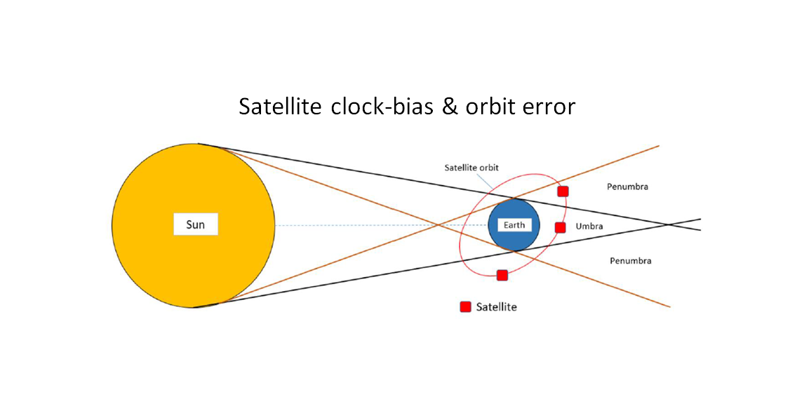
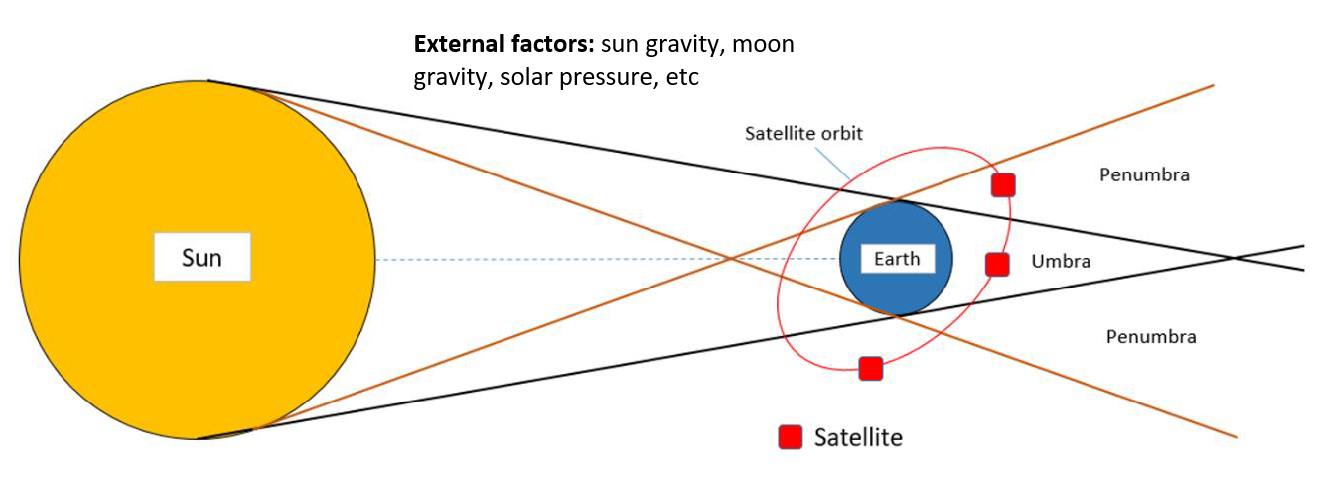
Meanwhile, the external factors that can affect the satellite clock-bias and orbit are solar radiation pressure and the effect of the Sun or Moon gravity. These factors affect the orbit and clock-bias by changing the dynamic states of satellites.

Solar radiation pressure is a force acting on the satellite’s surface caused by the sunlight and this force is proportional to the effective satellite surface area, to the reflectivity of the surface and to the solar flux.

Figure 2 shows the illustration of external factors affecting the dynamics of GNSS satellites.

In figure 2, it is shown that the position of the satellite with respect to the earth, Sun and Moon will affect how strong gravitational forces applied to the satellites and the umbra and penumbra satellite positions will affect how much solar radiation pressure applied to the satellites.

Figure 2: Illustration of external factors affecting the dynamics of satellites.

Accurate satellite clock-bias and orbit estimations

One solution to increase the accuracy of satellite clock-bias and orbit estimations is by applying corrections to the broadcasted clock-bias and orbit from GNSS navigation messages received at a receiver.

For a stand-alone receiver, the corrections should be performed at the local computing unit of the receiver without the need of internet connections (which is usually cannot be found in remote area).

Hence, the proposed solutions for stand-along and fast satellite clock-bias and orbit corrections are by using time-series deep learning modelling [1,2].

In the proposed solutions, a transformer-based neural network has been proposed to predict the correction of clock-bias and orbits given the broadcasted clock-bias and orbit from navigation messages. Transformer is a type of deep learning for time-series data.

In [1,2], there are two transformer model, each for clock-bias and orbit correction predictions. The model uses 12-hour of previous data to predict up to two-hour ahead of time. The prediction of corrections for up to two-hour can be done in few minutes.

The inputs of both transformer models consider both the internal and external factors affecting the dynamics of satellites, they are [1,2]:

- Internal factors: PRN identifies, date and time, broadcasted clock-bias or orbit (derived from ephemeris).

- External factors: The sun gravity factor (the one-over-square distance between a satellite and the Sun), the moon gravity factor (the one-over-square distance between a satellite and the Moon) and shadow function (describing whether the satellite is in or out shadow of the earth).

The next section will discuss the results of satellite clock-bias and orbit corrections predicted by the transformer model.

Satellite clock-bias correction

The results of the clock-bias correction performance of the transformer model are by comparing the correction with respect to the correction derived from international GNSS stations (IGS) rapid product [1].

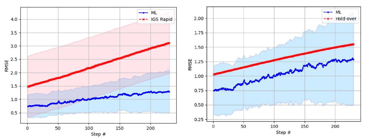
Figure 3 left shows the clock-bias correction between the transformer model predictions and IGS rapid derived predictions in a selected date and time.

The RMSE results on a selected date [1] from transformer correction predictions and IGS RAPID clock-bias correction estimate are (1.03 ± 1.1) ns and (2.29 ± 6.3) ns, respectively.

In figure 3 left, it can be observed that the transformer model corrections are noisier compared to the results from the IGS rapid predictions. One reason is that the transformer model also learns the noise from the data. In addition, a filtering process has been applied to the data from IGS rapid product.

In addition, figure 3 right shows the comparison between the transformer clock-bias correction prediction and hold-over method based on [3].

The holdover method is estimated as:

Where $𝑓$ is the carrier frequency, $\Delta f$ is the receiver clock drift, $𝑇$ is the receiver timing and $\Delta t$ is the clock-bias at the receiver. For this holdover, $𝑓=1575.42 𝑀𝐻𝑧$ that is the centre frequency of GPS L1 C/A signal and$ 𝑇=0$ 𝑡𝑜 $T=2 ℎ𝑟𝑠$ the prediction time (0-240 steps).

The main goal is that we want to estimate the $\Delta t$ as the clock-bias corrections. For the hold-over, we use $\Delta 𝑓=0.0229 𝑝𝑝𝑚~35 𝐻𝑧$ assuming an SV clock drift [4].

The RMSE results from the transformer predictions) and holdover clock estimate $(\Delta 𝑓=0.0229 𝑝𝑝𝑚~35 𝐻𝑧)$ are $(1.03 ± 1.1) ns$ and $1.3 ns$, respectively (see figure 3 right).

Since the hold-over results are estimated from the equation above, there is no variance from the holdover prediction.

Figure 3: (left) Comparison of clock correction between ML prediction and IGS RAPID clock estimation and (right) Comparison between transformer predictions and holdover estimation $\Delta 𝑓=0.0229 𝑝𝑝𝑚~35 𝐻𝑧$ (atomic clock).

Satellite orbit correction

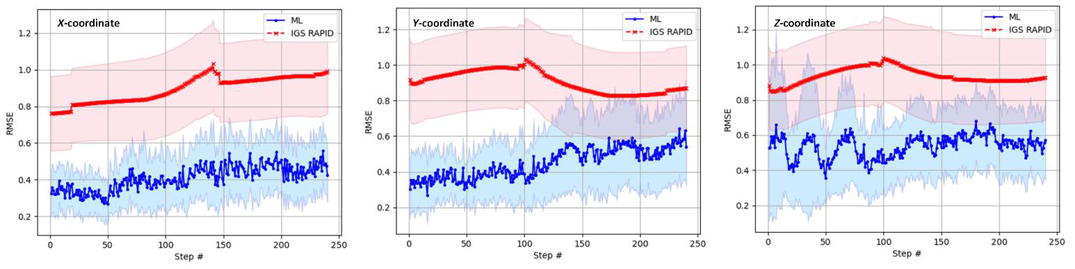
Similarly, the results of the satellite orbit correction performance of the transformer model are by comparing the correction with respect to the correction derived from IGS rapid product [2].

The RMSE results from the transformer corrections and IGS rapid derived correctios for X, Y and Z-coordinate corrections are:

For X-coordinate correction, the total RMSE for ML prediction is (0.33 ± 0.25) m and Total RMSE for IGS rapid prediction is (0.63 ± 0.52) m.

For Y-coordinate correction, the total RMSE for ML prediction is (0.31 ± 0.27) m and for IGS rapid prediction is (0.7 ± 0.46) m.

Finally, for Z-coordinate correction, the total RMSE for ML prediction is (0.35 ± 0.3) m and for IGS rapid prediction: (0.56 ± 0.43) m.

Figure 4: ML orbit prediction comparisons with IGS Rapid product for prediction date of 2018-02-15 for: (left) X-coordinate, (middle) Y-coordinate and (right) Z-coordinate.

Conclusion

In this post, we have discussed the importance of precise satellite clock-bias and orbit estimation and how these two values significantly affect the final calculated position of a GNSS receiver.

In real conditions, there are internal factors (such as satellite hardware and dynamic system) and external factors (such as solar pressure radiation, sun and moon gravity, etc) that cause deviation of estimate satellite clock-bias and orbit from its true or expected value.

To solve this, satellite clock-bias and orbit correction method have been proposed and discussed. The method leverages time series transformer model. The results of the correction estimate are also presented. The results show that the correction estimate can improve the estimate of satellite clock-bias and orbit and hopefully can improve the location estimate of a GNSS receiver in a standalone operation without any internet corrections.

References

[1] Syam, W.P., Priyadarshi, S., Roqué, A.A.G., Conesa, A.P., Buscarlet, G. and Orso, M.D., 2023, January. Fast and reliable forecasting for satellite clock bias correction with transformer deep learning. In Proceedings of the 54th Annual Precise Time and Time Interval Systems and Applications Meeting (pp. 76-96).

[2] Syam, W.P., Priyadarshi, S., Roqué, A.A.G., Conesa, A.P., Buscarlet, G. and Orso, M.D., 2023, September. Transformer deep learning for accurate orbit corrections in real-time. In Proceedings of the 36th International Technical Meeting of the Satellite Division of The Institute of Navigation (ION GNSS+ 2023) (pp. 159-174).

[3] Nicholls, C.W.T. and Carleton, G.C., 2004, August. Adaptive OCXO drift correction algorithm. In Proceedings of the 2004 IEEE International Frequency Control Symposium and Exposition, 2004. (pp. 509-517). IEEE.

[4] Kaplan, E.D. and Hegarty, C. eds., 2017. Understanding GPS/GNSS: principles and applications. Artech house.

You may find some interesting items by shopping here.

Understanding GPS/GNSS: Principles and Applications - a well-known handbook for GNSS