Applied programming

TUTORIAL: MATLAB software inter-connection and cooperation with PYTHON software using pyenv()

In a complex software application, most of the time, the application is written with several programming languages. These programming languages are inter-connected and cooperate together (compatible) to deliver the overall software functionalities.

Wahyudin Syam

Nov 29, 2023 • 12 min read

In this post, readers will understand and can implement a working example on how to write software in MATLAB and PYTHON that inter-connect and work together to deliver a machine learning capability.

The method for MALTAB-PYTHON interconnection uses pyenv() of MATLAB.

A machine learning (ML) model, that is neural network (NN) model, is written in Python by using PyTorch library. This NN model is trained in the python software.

Then, the MATLAB software will calculate inputs used for the NN model and call the NN model, written in Python, to perform prediction.

MATLAB and PYTHON connection

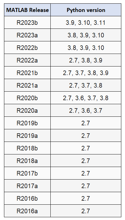
For MATLAB to communicate with Python, there should be a match version of MATLAB that is compatible with specific Python versions.

A detail list of Python versions that are compatible with MALTAB can be found here. Table 1 below shows the list of MATLAB-Python compatibility version.

It is important to note that, our MATLAB and Python version follow the compatibility list shown in table 1. Usually, the Python version will follow our MATLAB version since usually our MATLAB version is fixed since it is a licenced software.

Then, after knowing our MATLAB version, we can download the Python software that compatible with our MATLAB version.

Table 1: The list of MATLAB-Python compatibility version.

Case study: Machine learning application in MATLAB and PYTHON

In this case study to show MATLAB and Python interconnection and cooperation, a simple NN model is used.

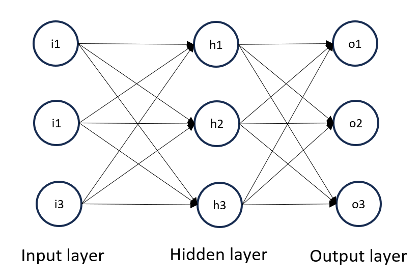
Figure 1 below shows the NN architecture. The NN architecture contains three inputs and three outputs as well as one hidden unit. The depth of the NN is three and the wide of NN is also three.

In figure 1, there are three layers on the NN: input, hidden and output layers. Each layer has three nodes.

Input layer requires three input values and output layer classifies given inputs into one of three possible classes.

Figure 1: The architecture of the NN model with three inputs and three outputs.

The Python code implementation uses PyTorch library as follows:

class NN(nn.Module):
    def __init__(self):
        super().__init__()
        self.flatten = nn.Flatten()       

        self.linear_relu_stack = nn.Sequential(
            nn.Linear(input_size, input_size),
            nn.ReLU(), 
            nn.Linear(input_size, input_size),
            nn.ReLU(),
            nn.Linear(input_size, 3)
        )
        
    def forward(self, x):
        x = self.flatten(x)
        out = self.linear_relu_stack(x)
        return out

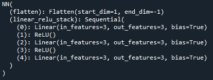
Figure 2 shows the created NN model.

Figure 2: The results of the implemented NN model.

In this case study, the inputs are generated by simulations. That are,

Inputs defined as class 1: three values, each normally generated with mean 1,2 and 3.
Inputs defined as class 2: three values, each normally generated with mean 7,8 and 8.
Inputs defined as class 3: three values, each normally generated with mean 11,12 and 13.

The implementation of these input generations, used to train the NN model, is as follows:

#Class 1
class_type=1

X_input_class_1a=np.random.normal(loc=1.0, scale=1.0, size=(n_data,1))
X_input_class_1b=np.random.normal(loc=2.0, scale=1.0, size=(n_data,1))
X_input_class_1c=np.random.normal(loc=3.0, scale=1.0, size=(n_data,1))

X_input_class_1=np.hstack([X_input_class_1a,X_input_class_1b,X_input_class_1c])

y_output_class_1=np.ones((n_data,1))*class_type


#Class 2
class_type=2

X_input_class_2a=np.random.normal(loc=7.0, scale=1.0, size=(n_data,1))
X_input_class_2b=np.random.normal(loc=8.0, scale=1.0, size=(n_data,1))
X_input_class_2c=np.random.normal(loc=9.0, scale=1.0, size=(n_data,1))

X_input_class_2=np.hstack([X_input_class_2a,X_input_class_2b,X_input_class_2c])

y_output_class_2=np.ones((n_data,1))*class_type


#Class 3
class_type=3

X_input_class_3a=np.random.normal(loc=11.0, scale=1.0, size=(n_data,1))
X_input_class_3b=np.random.normal(loc=12.0, scale=1.0, size=(n_data,1))
X_input_class_3c=np.random.normal(loc=13.0, scale=1.0, size=(n_data,1))

X_input_class_3=np.hstack([X_input_class_3a,X_input_class_3b,X_input_class_3c])

y_output_class_3=np.ones((n_data,1))*class_type

Practical example and codes of MATLAB and PYTHON inter-connection and cooperation

The fundamental goal of this case study is to implement the NN model in Python programming language for training and prediction phase. PyTorch library is used for the implementation of the NN model as well as to perform the training and prediction.

Meanwhile, the input calculations (the three-input required by the NN model) are calculated in MATLAB software.

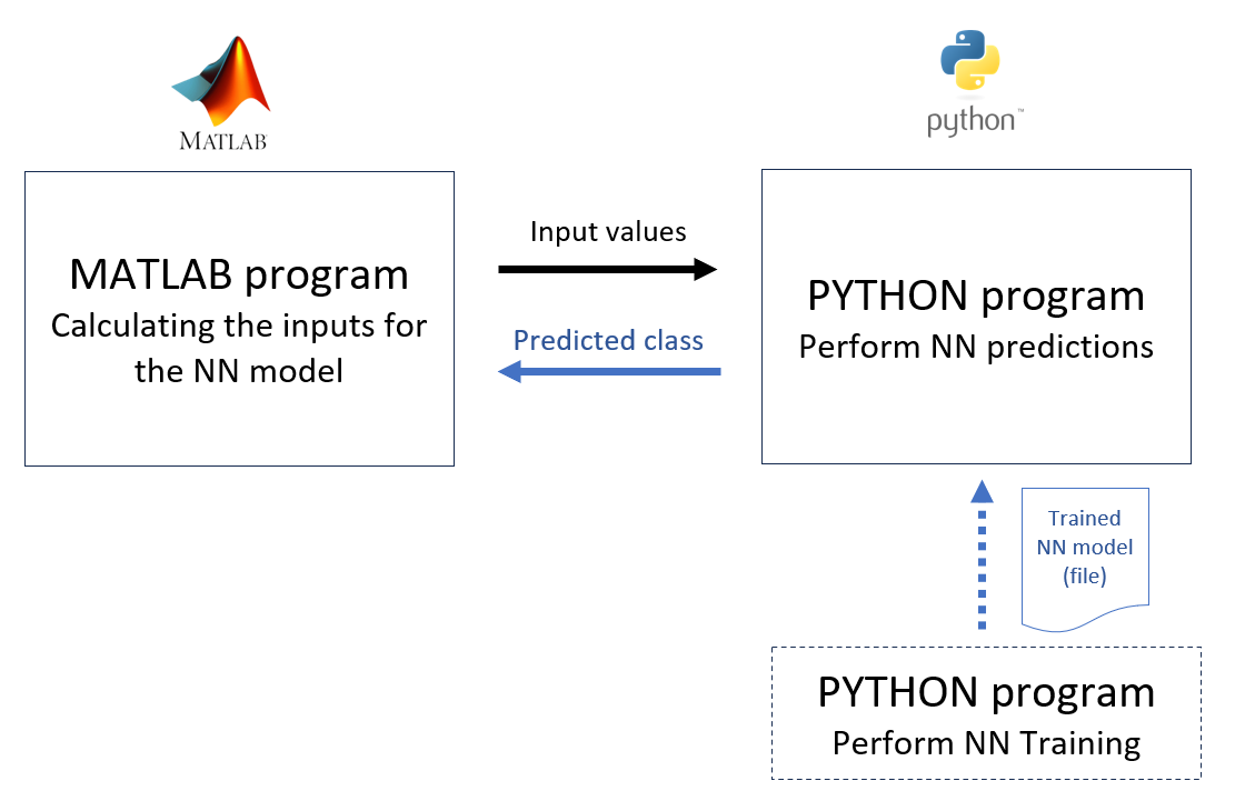
Figure 3 below shows the architecture of the MATLAB and Python interconnection. In figure 3, firstly, the NN model (implemented in Python) is trained independently. The result of this training process is a trained model in the form of a file “*.pth”.

Then, another Python software is written as the inference or prediction engine for the trained NN model. This Python software read the trained model file to perform inference.

The MATLAB software is then acting as an application software where it calculates “Features” (the NN inputs) and to predict the class of the calculated “features”.

To summarise, the overall operation of the software system is then as follow (figure 3). The application (the MATLAB software) calculates input features. These input features are then sent to the Python software to perform NN predictions. The predicted class (given in the inputs) is then sent back to the application (the MATLAB software).

One important note is that the Python software for NN predictions should be written as module.

Figure 3: MATAB-Python interconnection for the ML case study.

Training phase

The training phase uses 15000 of data. As being mentioned before, the data is simulated data generated from normal distributions.

The hyper-parameters for the training are as follows: batch size = 64, epoch = 20, loss function = cross-entropy (for classification task), optimiser = stochastic gradient descent and learning rate = 1e-3.

Important note is that, since the output layer has three nodes. Hence, the output should be converted into vector of three elements and the input and output variables should be converted into torch tensor format as follows:

for ii in range(len(y_train0)):
    if(y_train0[ii,0]==1):
        y_train[ii,0]=1
        y_train[ii,1]=0
        y_train[ii,2]=0
    elif(y_train0[ii,0]==2):
        y_train[ii,0]=0
        y_train[ii,1]=1
        y_train[ii,2]=0
    else:
        y_train[ii,0]=0
        y_train[ii,1]=0
        y_train[ii,2]=1
        
for ii in range(len(y_val0)):
    if(y_val0[ii,0]==1):
        y_val[ii,0]=1
        y_val[ii,1]=0
        y_val[ii,2]=0
    elif(y_val0[ii,0]==2):
        y_val[ii,0]=0
        y_val[ii,1]=1
        y_val[ii,2]=0
    else:
        y_val[ii,0]=0
        y_val[ii,1]=0
        y_val[ii,2]=1
        

#Convert numpy to Torch tensor
X_train=torch.from_numpy(X_train)
X_val=torch.from_numpy(X_val)
y_train=torch.from_numpy(y_train)
y_val=torch.from_numpy(y_val)

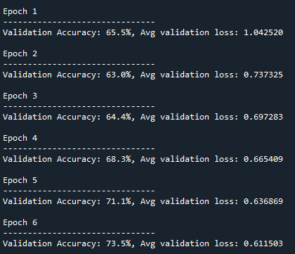
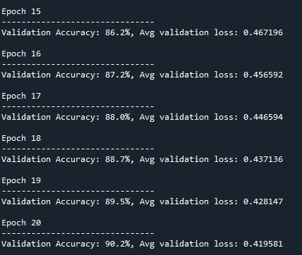
Figure 4 and figure 5 below shows the training accuracy at the initial and final epochs. At the end of the epoch, the training (validation) accuracy is about 90.2%.

Of course the accuracy can be improved by performing, for example, training with more data, larger or smaller batch size, bigger or smaller learning rate and other hyper-parameter settings.

Figure 4: Initial epochs of the NN training process.

Figure 5: Final epochs of the NN training process.

Prediction phase: MATLAB-Python interconnection

This section explains how MATLAB can interact with Python. The method used to connect MATLAB and Python is by using pyenv() function in MATLAB.

This pyenv() function opens connection to Python and establishes Python runtime environment inside a MATLAB session. This process is done only once in the same active MATLAB session.

The connection and establishment to Python is implemented as follows:

status=pyenv;
if(status.Status~="Loaded")%Connect to and load the python environment
	pyenv("Version",'C:\Users\WASY\AppData\Local\miniconda3\python.exe');%Only run once per MATLAB session
end

The if() clause is to make sure the connection is opened and established once during a MATLAB session. Remember that the MATLAB and PYTHON version should match each other.

For pyenv() method, the python should be implemented as module. The module here is that in the form of a function as follows:

def ML_prediction(X_input):

The Python module (in this case for NN model prediction) is imported and then loaded into the MATLAB session as follows:

ML_model=py.importlib.import_module('ML_prediction');
py.importlib.reload(ML_model);

Then, in MATLAB, inputs (to be then estimated its class type by the NN model) are generated as follows (in this case we generate inputs to be classified as class 2):

X_input_class_2a=randn()+7;
X_input_class_2b=randn()+8;
X_input_class_2c=randn()+9;

X_input_class_2=[X_input_class_2a,X_input_class_2b,X_input_class_2c];

ML_input=X_input_class_2;

And then, the ML prediction (performed by the Python software) is called and the class type result is received as follows:

val=ML_model.ML_prediction(ML_input);
val=double(val); %convert to MATLAB array (MATLAB variable)

In Python software for prediction, there is a little trick that we need to apply (maybe this is due to the MATLAB and PYTHON version) and to be able to process correctly input data sent from MATLAB.

This process is to separate the inputs sent from MATLAB to be still as an array of values in the Python prediction software instead of as a single value. The trick, to keep the MATLAB arrays still as an array in the Python software, is as follow:

X_input=X_input*1

The complete MATLAB and PYTHON software codes are provided in the next section.

Complete MATLAB and PYTHON code

The complete MATLAB code is as follow:

clear all;
close all;
clc;

% NOTE: MATLAB 2021a only support python 3.7 and 3.8

% LOAD the python interpreter (ONLY once per MATLAB session) --------------
status=pyenv;
if(status.Status~="Loaded")%Connect to and load the python environment
	pyenv("Version",'C:\Users\WASY\AppData\Local\miniconda3\python.exe');%Only run once per MATLAB session
end

% ML model loading --------------------------------------------------------
tic

ML_model=py.importlib.import_module('ML_prediction');
py.importlib.reload(ML_model);

% Input generation --------------------------------------------------------
%Generate input for class 2, expected ML prediction = class 2
X_input_class_2a=randn()+7;
X_input_class_2b=randn()+8;
X_input_class_2c=randn()+9;

X_input_class_2=[X_input_class_2a,X_input_class_2b,X_input_class_2c];

ML_input=X_input_class_2;

% ML Prediction -----------------------------------------------------------
val=ML_model.ML_prediction(ML_input);
val=double(val); %convert to MATLAB array (MATLAB variable)

processing_time_ML_prediction=toc; %Calculate the prediction time

if(val==0)
    fprintf("Class 1 detectted\n");    
elseif(val==1)
    fprintf("Class 2 detectted\n");    
else
    fprintf("Class 3 detectted\n");    
end

The complete Python code for ML training is as follow:

#ML Training

import numpy as np

#Scikit learn library
from sklearn.model_selection import train_test_split # Splitting the data set

#Pytorch machine learning library
import torch
from torch import nn
import torch.nn.functional as F

#Utilities
import time


############ Synthetic Data set generation ####################################
n_data=15000 #number of data points per class type

#Class 1
class_type=1

X_input_class_1a=np.random.normal(loc=1.0, scale=1.0, size=(n_data,1))
X_input_class_1b=np.random.normal(loc=2.0, scale=1.0, size=(n_data,1))
X_input_class_1c=np.random.normal(loc=3.0, scale=1.0, size=(n_data,1))

X_input_class_1=np.hstack([X_input_class_1a,X_input_class_1b,X_input_class_1c])

y_output_class_1=np.ones((n_data,1))*class_type


#Class 2
class_type=2

X_input_class_2a=np.random.normal(loc=7.0, scale=1.0, size=(n_data,1))
X_input_class_2b=np.random.normal(loc=8.0, scale=1.0, size=(n_data,1))
X_input_class_2c=np.random.normal(loc=9.0, scale=1.0, size=(n_data,1))

X_input_class_2=np.hstack([X_input_class_2a,X_input_class_2b,X_input_class_2c])

y_output_class_2=np.ones((n_data,1))*class_type


#Class 3
class_type=3

X_input_class_3a=np.random.normal(loc=11.0, scale=1.0, size=(n_data,1))
X_input_class_3b=np.random.normal(loc=12.0, scale=1.0, size=(n_data,1))
X_input_class_3c=np.random.normal(loc=13.0, scale=1.0, size=(n_data,1))

X_input_class_3=np.hstack([X_input_class_3a,X_input_class_3b,X_input_class_3c])

y_output_class_3=np.ones((n_data,1))*class_type



############# COMBINE ALL INPUTS and OUTPUTS ##################################

# COMBINED INPUT
input_size=3

X_input=np.vstack([X_input_class_1,X_input_class_2,X_input_class_3])


# COMBINED OUTPUT
y_output=np.vstack([y_output_class_1,y_output_class_2,y_output_class_3])

y_output=np.matrix(y_output) #convert to matrix form nx1



################## ML: Neural Network training ################################
start_time=time.time()

#training and validation data preparation
X_train, X_val, y_train0, y_val0 = train_test_split(X_input, y_output, random_state=3,train_size=0.8, shuffle=True)

#covert y vector into n x 2 matrix
y_train=np.zeros((len(y_train0),3))
y_val=np.zeros((len(y_val0),3))

for ii in range(len(y_train0)):
    if(y_train0[ii,0]==1):
        y_train[ii,0]=1
        y_train[ii,1]=0
        y_train[ii,2]=0
    elif(y_train0[ii,0]==2):
        y_train[ii,0]=0
        y_train[ii,1]=1
        y_train[ii,2]=0
    else:
        y_train[ii,0]=0
        y_train[ii,1]=0
        y_train[ii,2]=1
        
for ii in range(len(y_val0)):
    if(y_val0[ii,0]==1):
        y_val[ii,0]=1
        y_val[ii,1]=0
        y_val[ii,2]=0
    elif(y_val0[ii,0]==2):
        y_val[ii,0]=0
        y_val[ii,1]=1
        y_val[ii,2]=0
    else:
        y_val[ii,0]=0
        y_val[ii,1]=0
        y_val[ii,2]=1
        

#Convert numpy to Torch tensor
X_train=torch.from_numpy(X_train)
X_val=torch.from_numpy(X_val)
y_train=torch.from_numpy(y_train)
y_val=torch.from_numpy(y_val)


############## Neural network arhitecture #####################################
batch_size = 64

device="cpu"

# Define model
class NN(nn.Module):
    def __init__(self):
        super().__init__()
        self.flatten = nn.Flatten()       

        self.linear_relu_stack = nn.Sequential(
            nn.Linear(input_size, input_size),
            nn.ReLU(), 
            nn.Linear(input_size, input_size),
            nn.ReLU(),
            nn.Linear(input_size, 3)
        )
        
    def forward(self, x):
        x = self.flatten(x)
        out = self.linear_relu_stack(x)
        return out

model = NN().to(device)
print(model)

# calcate model parameters
print("\n")

pytorch_total_params = sum(p.numel() for p in model.parameters())
print("Total model parameters: ", pytorch_total_params)
pytorch_trainable_params = sum(p.numel() for p in model.parameters() if p.requires_grad)
print("Trainable model parameters: ", pytorch_trainable_params)

print("\n")



############## DEFINE Training process ########################################
loss_fn = nn.CrossEntropyLoss() #performs softmax internally, so we can directly pass in the model's outputs
optimizer = torch.optim.SGD(model.parameters(), lr=1e-3)


#Train
def train(X_train, y_train, model, loss_fn, optimizer):
    size = len(X_train)
    model.train()
    
    num_batches=int(np.floor(size/batch_size))
    
    for ii in range(num_batches):
        X, y = X_train[ii*batch_size:ii*batch_size+batch_size].to(device), y_train[ii*batch_size:ii*batch_size+batch_size].to(device)

        X.float()
        y.float()
        
        # Compute prediction error
        pred = model(X.float())      
        loss = loss_fn(pred, y) #performs softmax internally, so we can directly pass in the model's outputs
       
        # Backpropagation
        loss.backward()
        optimizer.step()
        optimizer.zero_grad()

        if (ii % num_batches) == 0:
            loss, current = loss.item(), (ii + 1) * len(X)
            
            
#Test
def test(X_val,y_val, model, loss_fn):
    size = len(X_val)
    num_batches =int( np.floor(size/batch_size))
    model.eval()
    test_loss, correct = 0, 0
    with torch.no_grad():
        for ii in range(num_batches):
            X, y = X_val[ii*batch_size:ii*batch_size+batch_size].to(device), y_val[ii*batch_size:ii*batch_size+batch_size].to(device)
            
            X.float()
            y.float()
                    
            pred = model(X.float())            
     
            test_loss += loss_fn(pred, y).item()
     
            correct += (pred.argmax(1) == y.argmax(1)).type(torch.float).sum().item() #Check that the max value is at the same index
                    
                
    test_loss /= num_batches
    correct /= size
    print(f"Validation Accuracy: {(100*correct):>0.1f}%, Avg validation loss: {test_loss:>8f} \n")
    
    
#Processing training
epochs = 20
for t in range(epochs):
    print(f"Epoch {t+1}\n-------------------------------")
    train(X_train,y_train, model, loss_fn, optimizer)
    test(X_val,y_val, model, loss_fn) # In this case, the test is Validation
print("Done!")

total_time=(time.time()-start_time)/60 #in minute
print("total time: ", total_time)


#################### SAVING the trained model #################################
model_filename="ML_model.pth"
torch.save(model.state_dict(), model_filename)
print("Saved PyTorch Model State to ML_model.pth")

The complete Python code for ML prediction is as follow:

# ML Prediction as a Python module

import numpy as np


#Pytorch machine learning library
import torch
from torch import nn

    
def ML_prediction(X_input):
    
    X_input=X_input*1
    
    n_input=len(X_input)
    
    input_size=n_input
    
    # Define model ----------------------------------------------------------------
    class DNN(nn.Module):
        def __init__(self):
            super().__init__()
            self.flatten = nn.Flatten()
                  
            self.linear_relu_stack = nn.Sequential(
                nn.Linear(input_size, input_size),
                nn.ReLU(), 
                nn.Linear(input_size, input_size),
                nn.ReLU(),
                nn.Linear(input_size, 3)
            )             
                   

        def forward(self, x):
            x = self.flatten(x)
            out = self.linear_relu_stack(x)
            return out
    
    
    # LOADING the trained model -----------------------------------------------
    model_filename = "ML_model.pth"
    
    device="cpu"
    model = DNN().to(device)  
    model.load_state_dict(torch.load(model_filename))
    
    # PERFORM prediction ------------------------------------------------------
    ML_input=X_input
    
    ML_input=np.matrix(ML_input)
            
    ML_input=torch.from_numpy(ML_input)
    
    ML_input.to(device)
    
    ML_input.float()
    
    model.eval()
    
    with torch.no_grad():
        pred = model(ML_input.float()) 
        
    #Give the class prediction ------------------------------------------------
    pred=pred.argmax(1) #The class is the column index of array "pred": 0 or 1 or 2
     
    class_prediction=pred.numpy()

    return class_prediction

Conclusion

In this post, a software ecosystem containing MATLAB and PYTHON software is presented. The connection and cooperation between MATLAB and PYTHON are demonstrated by using a case study of Neural Network classification problems.

In real complex software applications, many of the software are not written in a single programming language. Instead, the software is written using several programming languages to perform a specific function that is best using a specific programming language.

Python, with the PyTorch library, is very famous to be used for machine learning applications. In the case study presented in this post, a software application (written in MATLAB) calculates “features”, connects and sends data to an ML software (written in Python) to receive the type of class of the “features”. The classification or prediction is performed in the python software.

You may find some interesting items by shopping here.